Anomaly Detection Overview
Anomaly detection identifies unexpected behavior in telemetry data — patterns that differ significantly from what is considered normal. These anomalies can indicate system malfunctions, equipment degradation, security breaches, or operational inefficiencies.
How It Works
Section titled “How It Works”Trendz anomaly detection is unsupervised — it requires no manual thresholds or labeled training data. Instead, it learns what “normal” looks like from historical telemetry and then scores deviations in new data automatically.
The typical workflow:
- Build Anomaly Detection Model — configure input scope, choose a detection strategy, and train the model on historical telemetry.
- Explore results — review detected anomalies per device using the activity heatmap, ranked item table, and cluster analysis.
- Set up continuous monitoring — enable periodic scanning so the model keeps detecting anomalies as new data arrives.
- Enable alarms — automatically trigger ThingsBoard alarms when anomaly scores exceed defined thresholds.
The default setup takes under 2 minutes and requires no ML expertise. Advanced users can also fine-tune clustering algorithms, segmentation, distance functions, and scoring thresholds directly.
Key Metrics
Section titled “Key Metrics”Trendz anomaly detection is based on two core metrics:
| Metric | Description |
|---|---|
| Anomaly Score | A numeric value representing how far a data segment deviates from expected (normal) behavior. Measures the intensity of the anomaly. |
| Anomaly Score Index | A composite metric that combines anomaly score with the duration of the anomaly. Helps prioritize anomalies that have a greater cumulative impact over time. |
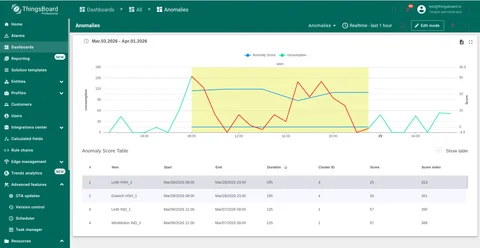
Example — pump vibration analysis:
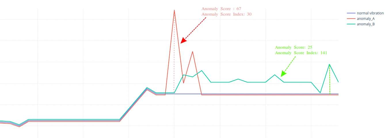
- Anomaly A — a sharp vibration spike lasting ~5 seconds. High anomaly score, but short duration keeps the score index low.
- Anomaly B — a longer-lasting deviation without large spikes. Lower anomaly score, but the score index is higher due to extended duration — suggesting greater long-term impact on pump health.
Use Anomaly Score to detect sharp, short-term deviations. Use Anomaly Score Index to surface sustained anomalies that may cause greater damage over time.
Trendz Anomaly Detection
Section titled “Trendz Anomaly Detection”Trendz covers the full anomaly detection lifecycle — from building and training a model to analyzing results, setting up continuous monitoring, and embedding insights into ThingsBoard dashboards. Explore the capabilities below.
-
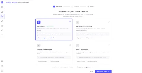
Create Anomaly Model
Choose a detection intent, configure input scope and sensitivity, then build your first model in minutes.
-
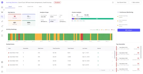
Analyze Anomalies
Review detected anomalies per device using the activity heatmap, ranked item table, and cluster analysis to assess model quality and prioritize issues.
-
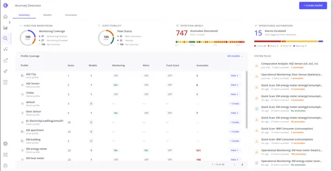
Anomaly Detection Interface
Explore the Summary, Models, and Anomalies tabs — fleet-wide KPIs, full model list, and a unified view of all detected anomaly events.
-
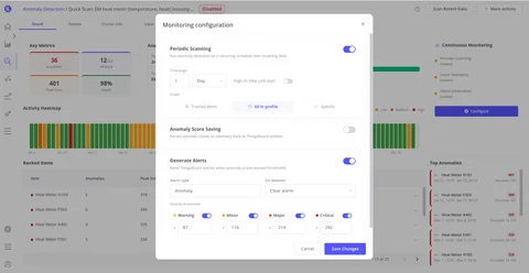
Set Up Monitoring
Enable periodic scanning, configure anomaly score saving, and automatically generate ThingsBoard alarms when anomaly scores exceed defined thresholds.
-
Visualize Anomalies
Embed anomaly data in ThingsBoard dashboards using Anomaly View Reports, Anomaly Fields in custom views, or Business Entity Fields for saved telemetry.
-
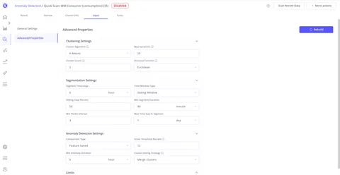
Advanced Properties
Fine-tune clustering algorithms, segmentation window settings, score thresholds, and anomaly detection parameters for full control over model behavior.
Was this helpful?