Prediction
Trendz provides built-in tools for time-series prediction, letting you create predictive models with minimal data science background. Data filtering, normalization, and model training are all handled automatically in the background.
You can enable predictions for any data field, including calculated fields. Typical use cases include:
- Energy forecasting — estimate consumption for the upcoming quarter or year
- Maintenance scheduling — predict optimal maintenance windows
- Failure prediction — anticipate the next potential system failure
- Manufacturing KPIs — forecast key performance indicators and their relation to current system state
- Resource management — calculate time until a resource (e.g. fuel tank) is depleted
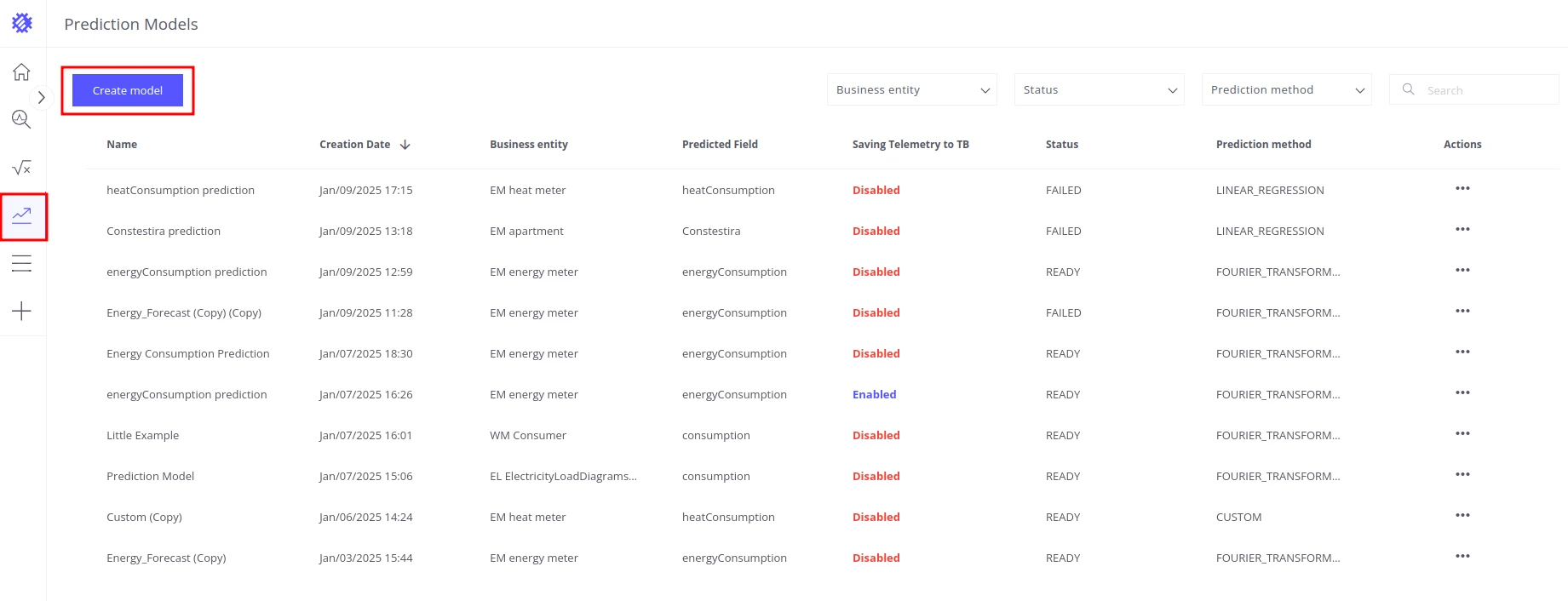
Accessing Prediction Models
Section titled “Accessing Prediction Models”Click the Prediction Models icon in the left sidebar to open the models section. The table lists all existing prediction models with their key details. To create a new forecast, click Create model.
Input tab
Section titled “Input tab”The Input tab configures all settings needed to generate forecasts.
General Settings
Section titled “General Settings”| Field | Description |
|---|---|
| Entity | The entity type for which the prediction is performed. |
| Predicted Field | The specific field to forecast (e.g. energy consumption, temperature). |
| Item | One or more specific devices or assets to focus the analysis on. Multiple items can be selected. |
| Key | The identifier under which predicted telemetry is saved in ThingsBoard, prefixed with _EPD_. For example, setting the key to energy_forecast stores telemetry under _EPD_energy_forecast. The prefix ensures predicted values never overwrite existing ThingsBoard telemetry. |
| Timerange for Model Training | The historical data period used for training (e.g. last 3 months, last year). |
| Prediction Range | How far into the future the model predicts (e.g. 3). |
| Prediction Unit | The time unit for the prediction range: Hours, Days, Weeks, Month. |
Prediction Method
Section titled “Prediction Method”Select the algorithm that best fits your data characteristics. Each method includes a short in-UI description.
| Method | Best for |
|---|---|
| Fourier Transformation | Data with cyclic trends and seasonal patterns — decomposes the series into its frequency components. |
| Prophet | Time series with strong seasonality and holiday effects; uses an additive model of trend + seasonality + holidays. |
| Multivariable Prophet | Multiple interconnected time series that should be predicted simultaneously. |
| ARIMA | Series with trends and seasonal variation; combines autoregressive and moving-average components. |
| Linear Regression | Predicting a dependent variable from one or more independent variables via a linear relationship. |
| Custom Model | Arbitrary multivariable predictions using any Python library; you supply the model source and Trendz handles data injection and output processing. On self-hosted installations you can install additional Python packages to extend the available libraries. See Custom Python models. |
Segment Strategy
Section titled “Segment Strategy”Before training, Trendz divides input telemetry into segments — equal-length time ranges that cover the full training period. Segments are used iteratively for model fitting, prediction building, and accuracy calculation.
  FIXED — sequential, no gaps, no overlaps  ──────────────────────────────────────────▶ time  ╔════════╗╔════════╗╔════════╗╔════════╗  ║ seg 1  ║║ seg 2  ║║ seg 3  ║║ seg 4  ║  ╚════════╝╚════════╝╚════════╝╚════════╝
  SLIDING_WINDOW_UNIT — overlapping, step < segment size  ──────────────────────────────────────────▶ time  ╔════════╗  ║ seg 1  ║  ╚════════╝       ╔════════╗       ║ seg 2  ║       ╚════════╝            ╔════════╗            ║ seg 3  ║            ╚════════╝
STICK_TO_END — only the last N segments are used ──────────────────────────────────────────▶ time ░░░░░░░░░░░░░░░╔════════╗╔════════╗╔════════╗ (excluded) ║ seg 1 ║║ seg 2 ║║ seg 3 ║ ╚════════╝╚════════╝╚════════╝| Strategy | Description |
|---|---|
| AUTO | Trendz automatically analyzes the data and determines the optimal segmentation. Use this if you are unsure which strategy suits your task. |
| FIXED | Divides data sequentially from start to end with no gaps or overlaps. A 120-day range with 10-day segments produces 12 segments. |
| SLIDING_WINDOW_UNIT | Like FIXED, but segments overlap. The step size is defined in time units. A 120-day range with 10-day segments and a 5-day step produces 23 segments, each overlapping its neighbors. |
| SLIDING_WINDOW_PERCENT | Like SLIDING_WINDOW_UNIT, but the step is a percentage of the segment size. A 20% step on a 10-day segment equals a 2-day step. |
| STICK_TO_END | Like FIXED, but only uses the last N segments from the end of the training range. Useful for focusing training on the most recent data. |
Include Last Unfinished Segment — when enabled, Trendz includes any partial segment at the end of the training range that does not fill a full segment length. Disable this if partial segments would cause overfitting.
Aggregation Settings
Section titled “Aggregation Settings”These settings preprocess data before it is fed into the prediction model:
| Setting | Description |
|---|---|
| Aggregation | How input data is summarized: AVG, SUM, LATEST, MIN, MAX, COUNT, UNIQ, and others. |
| Grouping Interval | The time bucket for aggregation: hour, day, week, month. |
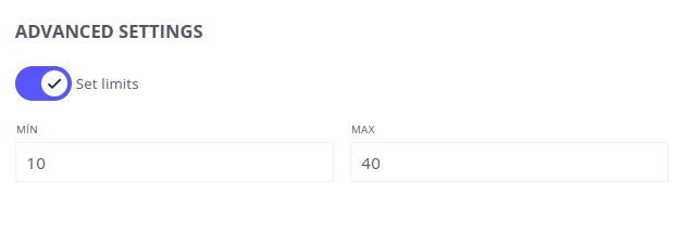
Advanced Settings
Section titled “Advanced Settings”Enable Set Limits to constrain predicted values to a defined range. Enter the minimum and maximum values to serve as prediction boundaries.
Example: For a water temperature model, setting MIN to 0 and MAX to 100 ensures all predicted values stay within 0°C–100°C.
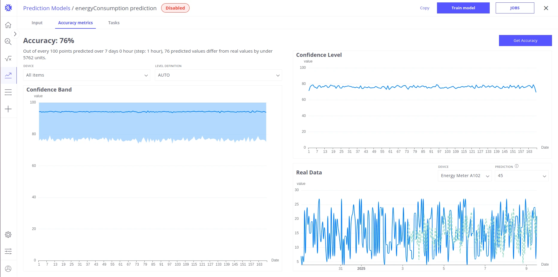
Accuracy tab
Section titled “Accuracy tab”After training, the Accuracy tab lets you validate how well the model performs. You must configure the evaluation parameters before calculating accuracy.
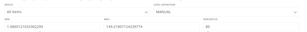
Configuration
Section titled “Configuration”- Select the device(s) to evaluate.
- Choose how thresholds are determined:
- AUTO — Trendz analyzes your prediction data and fills the required fields automatically.
- MANUAL — You provide the threshold values for each metric.
- Click Get Accuracy.
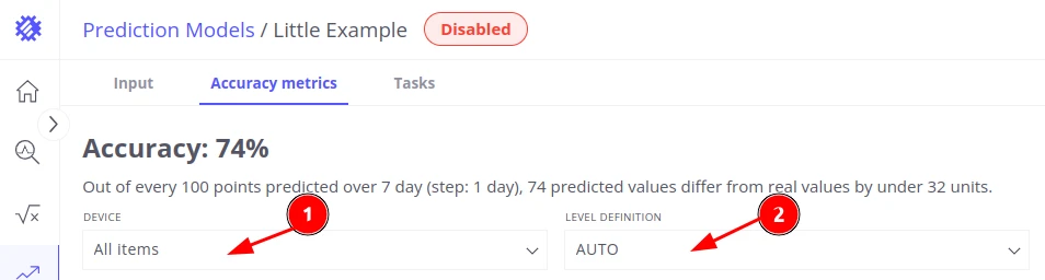
Accuracy Summary
Section titled “Accuracy Summary”Provides an overall percentage score describing how closely the predicted values align with actual telemetry.
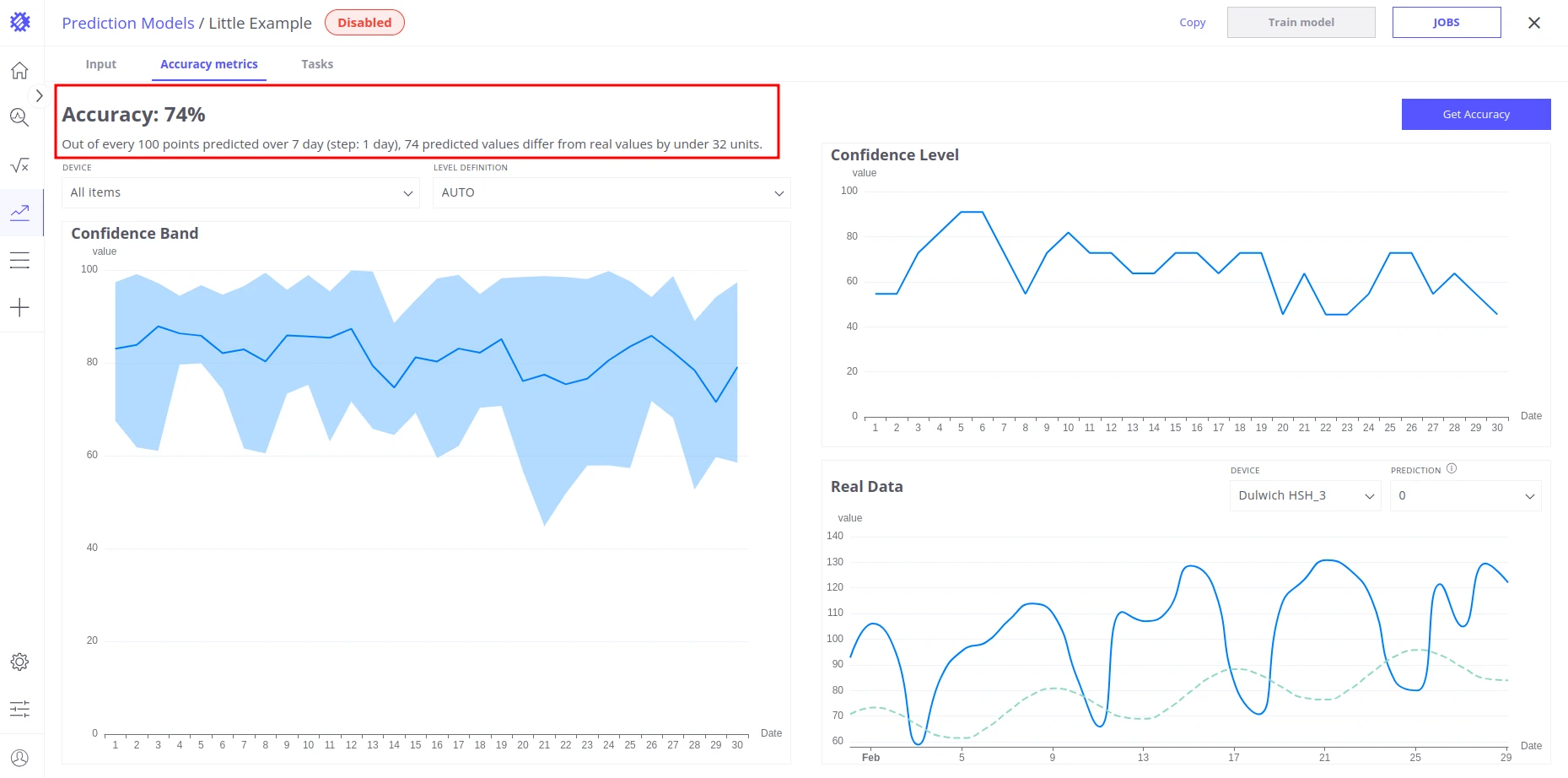
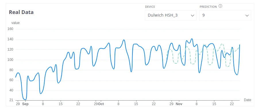
Real Data
Section titled “Real Data”Displays predicted data for a selected segment alongside the corresponding original historical telemetry.
Parameters:
- Device Name — the device to inspect
- Segment Number — the segment whose data to display
Confidence Level
Section titled “Confidence Level”Shows prediction accuracy as a binary metric per time unit. A time unit is marked true if both the value difference and the time offset between expected and actual values are within the configured thresholds; otherwise false. Results are aggregated across all segments.
Parameters:
- Acceptable Value Error — maximum allowable difference between predicted and actual values
- Acceptable Time Error — maximum allowable time offset between predicted and actual values
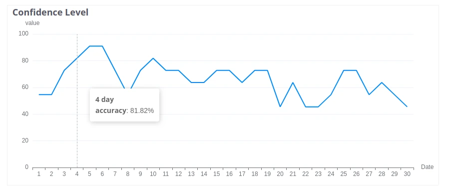

Example: You predict remaining fuel level over 14 days. Setting Acceptable Value Error to 20 (L) and Acceptable Time Error to 2 (hours) means a predicted value of 80 L is marked correct if the actual reading is within ±20 L of 80 at the predicted time, or equals 80 within a 2-hour window.
Confidence Band
Section titled “Confidence Band”Shows accuracy as a continuous percentage difference (error function) between predicted and actual values, measured per time unit within each segment. The min, max, and average (displayed on the chart) are aggregated across all segments for the selected percentile of best values.
Parameters:
- MIN — minimum possible telemetry value (defines the full value range)
- MAX — maximum possible telemetry value (defines the full value range)
- PERCENTILE — the percentile of best values to include when aggregating results
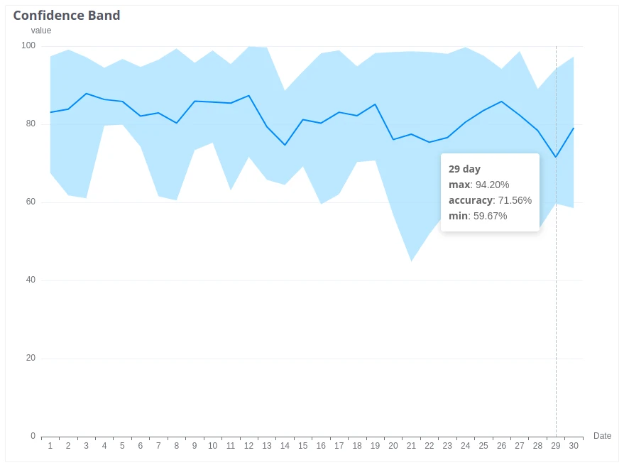
Example: An energy meter reports consumption between 0 and 50 kWh. Setting MIN to 0 and MAX to 50 means the full error range is 50 kWh. If the predicted value is 25 kWh and the actual reading is 30 kWh, the error is 5/50 = 10%, so accuracy is 90%.
Tasks tab
Section titled “Tasks tab”The Tasks tab lists all jobs initiated for this model, including their current status (completed, in progress, pending). For full task management details, see the Tasks Service documentation.
Example: Forecasting energy consumption for a building
Section titled “Example: Forecasting energy consumption for a building”This example creates a 3-month energy consumption forecast. The dataset includes Buildings, Apartments, and energy meters installed in each Apartment. Telemetry is aggregated from sensors at the building level.
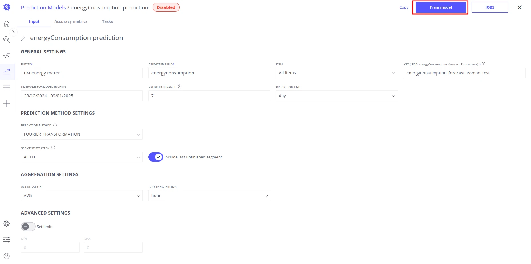
Configure and train the model
Section titled “Configure and train the model”Input tab:
| Setting | Value |
|---|---|
| Entity | Energy meter |
| Predicted Field | energyConsumption |
| Item | Energy Meter H101 |
| Key | Energy_Meter_H101 |
| Timerange for Model Training | Last Year |
| Prediction Range | 3 |
| Prediction Unit | Month |
Prediction Method:
| Setting | Value |
|---|---|
| Prediction Method | FOURIER_TRANSFORMATION |
| Segment Strategy | AUTO |
Aggregation:
| Setting | Value |
|---|---|
| Aggregation | AVG |
| Grouping Interval | DAY |
Name the model energyConsumption prediction, then click Train Model in the upper-right corner. Once training completes, open the Accuracy tab to evaluate the model’s performance. If training fails, Trendz raises an error — check the model configuration and ensure the training time range contains sufficient data.
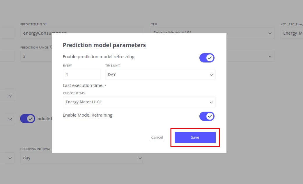
Save predicted telemetry to ThingsBoard
Section titled “Save predicted telemetry to ThingsBoard”If the accuracy is satisfactory, enable the prediction job to write results back to ThingsBoard:
- Click JOBS in the upper-right corner to open the Prediction Model Parameters modal.
- Enable Enable prediction model refreshing.
- Set the refresh interval, for example: EVERY 1 DAY.
- Select the items to run predictions for (e.g. Energy Meter H101).
- Enable Enable Model Retraining so the model retrains automatically when new data arrives.
- Click Save.
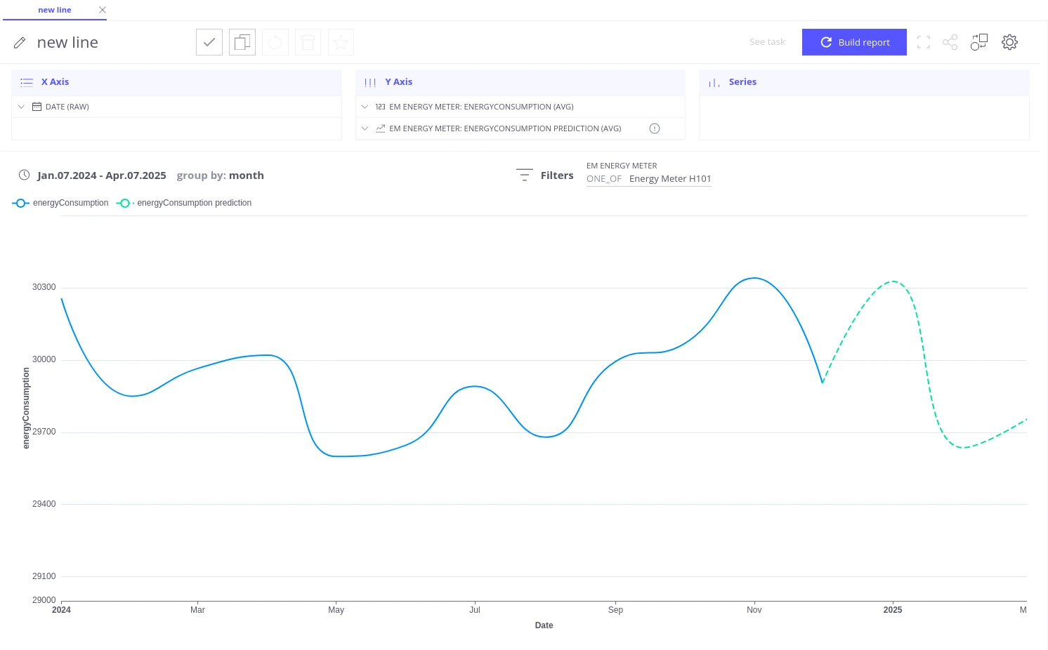
Visualize the forecast in a line chart
Section titled “Visualize the forecast in a line chart”- Go to View Fields and select a Line Chart view.
- Add Date (RAW) as the X-axis.
- Add
energyConsumptiontelemetry as the Y-axis. - Add
energyConsumptionprediction telemetry as a second Y-axis series. - Add the energy meter field to the Filter section and select Energy Meter H101.
- Set the date range to cover both historical and predicted data (e.g. 07/01/2024–07/04/2025).
- Click Build report.
Was this helpful?