Anomaly Model Properties
The Properties tab is where you configure the anomaly model before building it. It is organized into two sections in the left panel: General Settings and Advanced Properties.
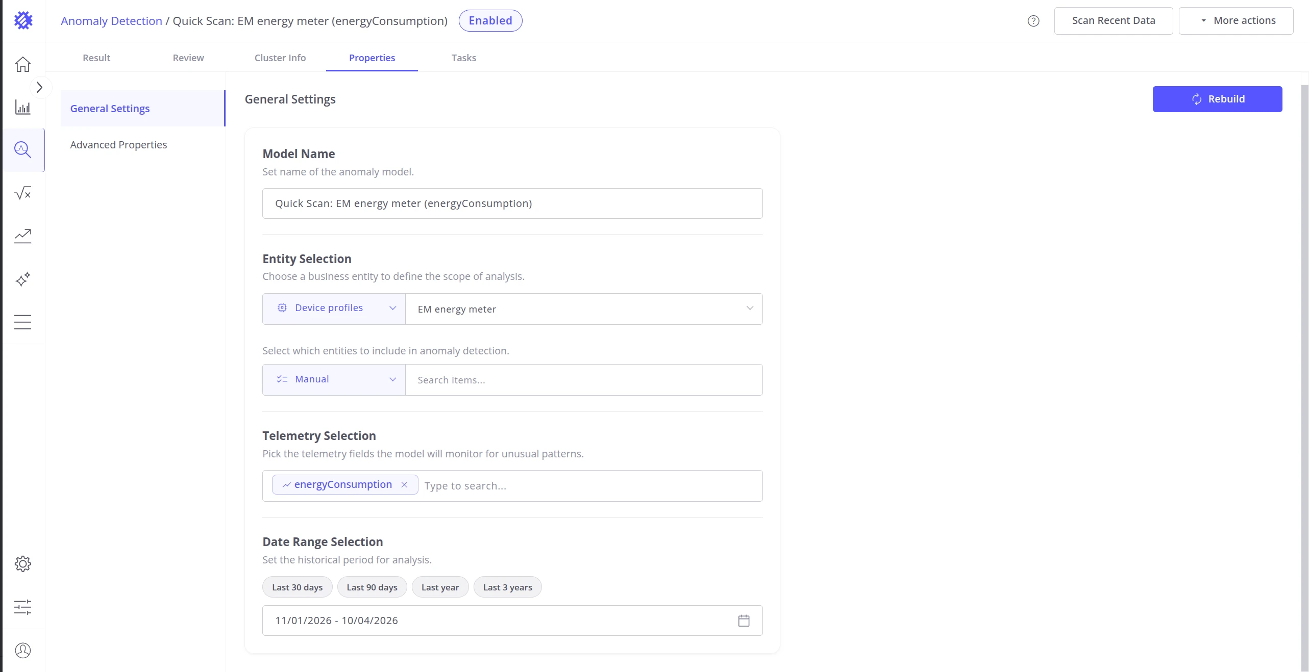
General Settings
Section titled “General Settings”General settings define the data scope used for training.
| Setting | Description |
|---|---|
| Model Name | Display name for the anomaly model. |
| Entity | The entity type for which anomaly detection will be performed. |
| Fields | Numeric telemetry fields to analyze, e.g. temperature, vibration, energy consumption. All fields must belong to the same entity type — combining fields from different entity types is not supported. |
| Items | Specific devices or assets to include in training. Use the most representatively normal items for better accuracy. |
| Time Range | Historical data period to use for training, e.g. past 3 months or 1 year. |
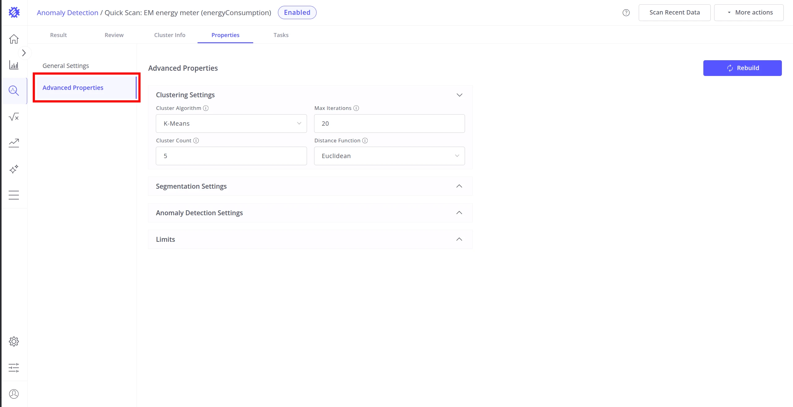
Advanced Properties
Section titled “Advanced Properties”Trendz uses unsupervised machine learning for anomaly detection — no labeled data or pre-defined fault conditions are required. The model learns what “normal” looks like from historical telemetry and flags deviations automatically.
Raw telemetry │ ▼ ┌────────────────┐ │ Segmentation │ Split data into fixed-length windows └────────┬───────┘ │ ▼ ┌────────────────┐ │ Normalization │ Scale values for comparability └────────┬───────┘ │ ▼ ┌────────────────┐ │ Feature extract│ Describe the shape of each segment └────────┬───────┘ │ ▼ ┌────────────────┐ │ Clustering │ Group segments into "normal" clusters └────────┬───────┘ │ ▼ ┌────────────────────────────────┐ │ Anomaly Score = distance from │ │ nearest cluster centroid │ └────────────────────────────────┘- Segmentation — continuous telemetry is split into fixed-length time windows. Configure window size, type, and gap tolerances in Segmentation Settings.
- Normalization — values within each segment are scaled automatically so that fields with different units and ranges can be compared fairly.
- Feature extraction — each segment is described either by statistical attributes (mean, std, slope) or by its overall shape. Configure the representation in Anomaly Detection Settings.
- Clustering — segments are grouped into clusters representing distinct normal operating behaviors. Choose the algorithm and tune its parameters in Clustering Settings.
- Anomaly scoring — each segment receives a score equal to its distance from the nearest cluster centroid. Configure the score threshold and filtering in Anomaly Detection Settings.
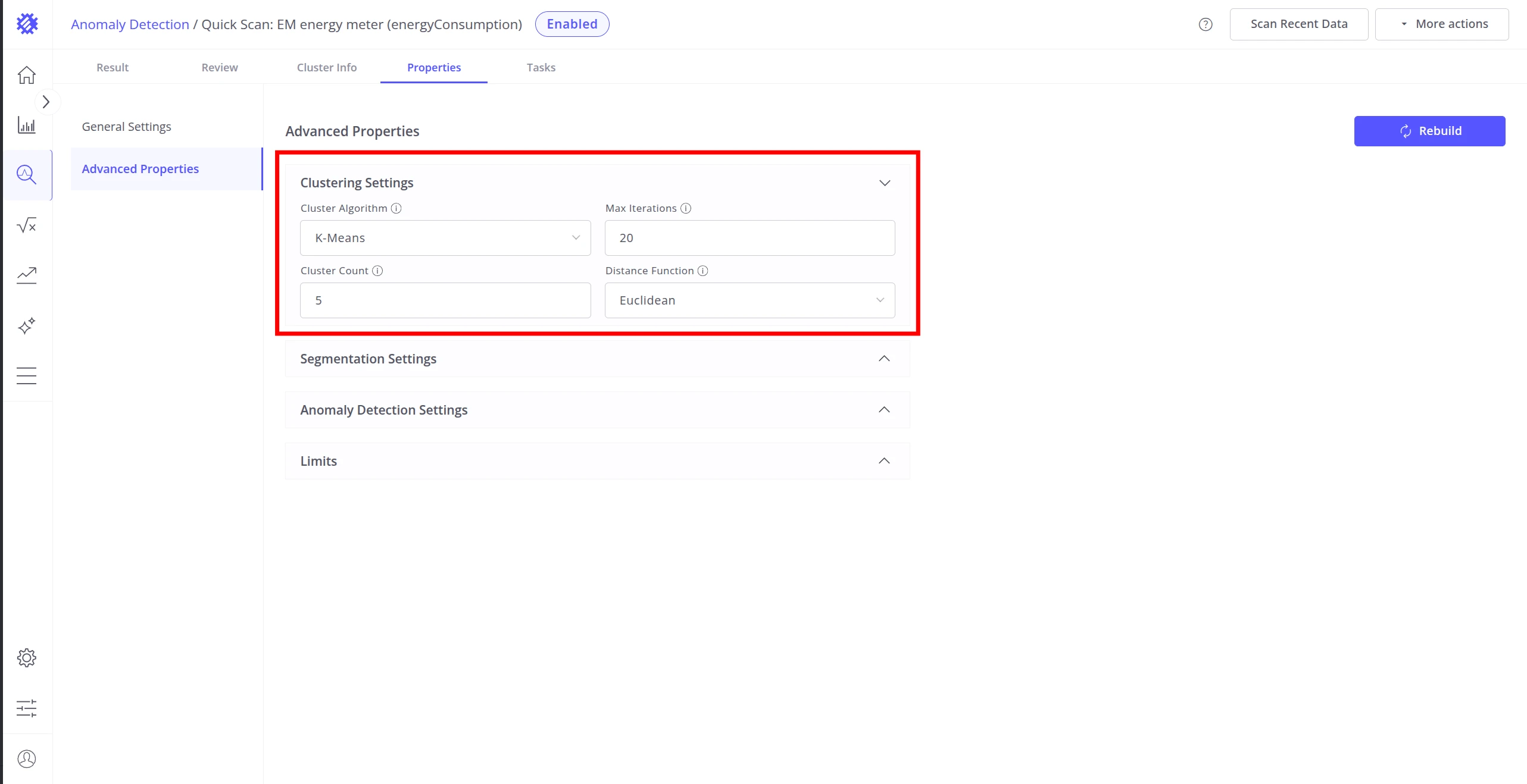
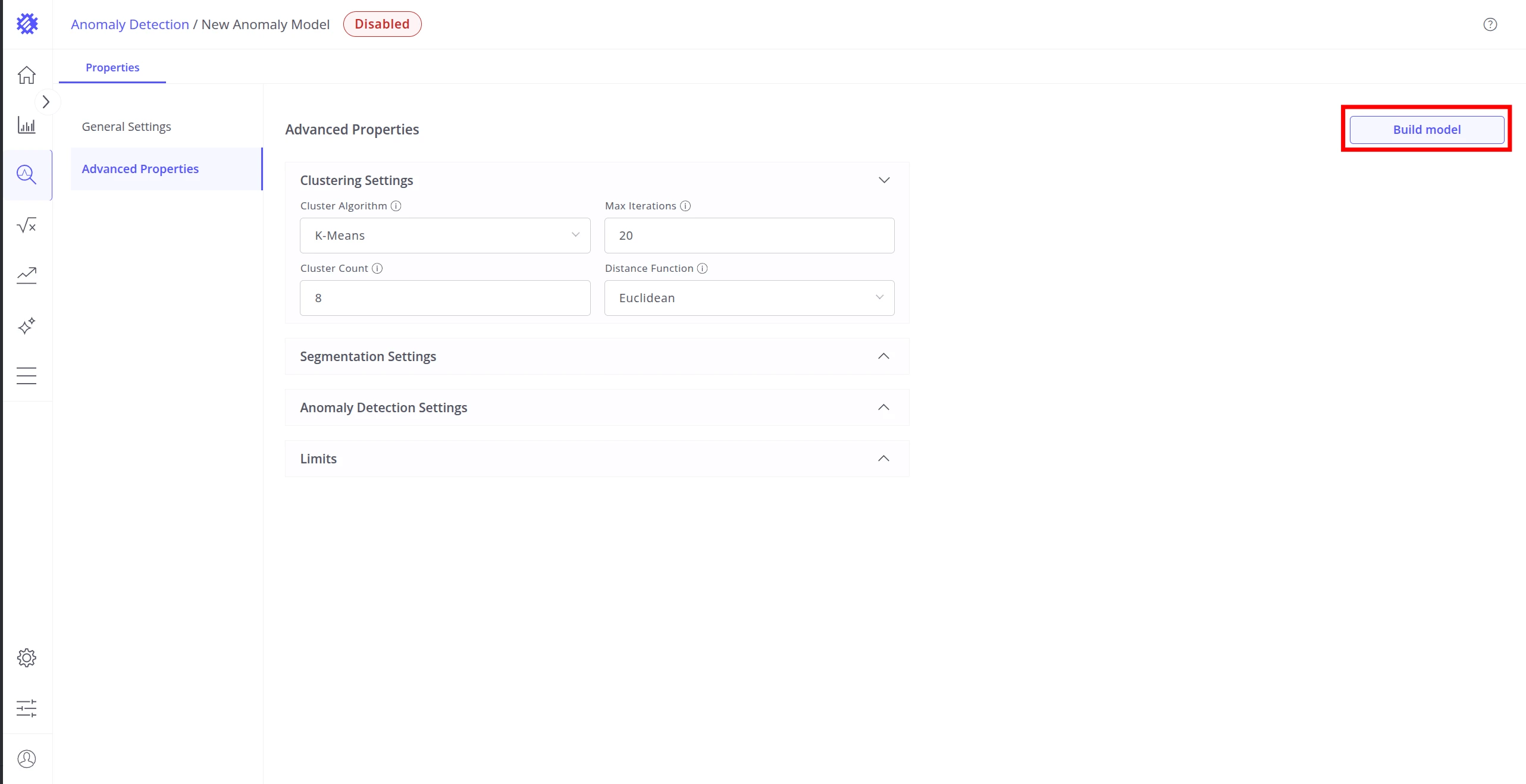
Clustering Settings
Section titled “Clustering Settings”Clustering settings determine which algorithm groups data segments into “normal” clusters. Anomalies are segments that don’t fit well into any cluster.
Segments │ ├── K-Means ──────▶ Fixed # of spherical clusters │ Anomaly = far from centroid │ Best for: clean, consistent data │ ├── DBSCAN ───────▶ Density-based clusters, any shape │ Anomaly = isolated / low-density point │ Best for: noisy data, varied shapes │ └── GMM ──────────▶ Probabilistic mixture of Gaussians Anomaly = low probability point Best for: flexible, overlapping clusters| Setting | Description |
|---|---|
| Cluster Algorithm | K-Means, DBSCAN, or GMM (Gaussian Mixture Model). |
| Cluster Count | Number of clusters to create (K-Means and GMM). Set this to the number of distinct typical operating behaviors in your data — for example, use 3 if your equipment has three recognizable normal states. |
| Max Iterations | How many refinement passes K-Means performs. |
| Max Epsilon | DBSCAN — maximum distance between points to be considered neighbours. |
| Min Points in Cluster | DBSCAN — minimum neighbours needed to form a valid cluster. |
| Distance Function | How similarity between segments is measured: DTW (handles similar shapes with different timing), Euclidean (straight-line), Chebyshev (largest single difference), Manhattan (sum of differences), or Canberra (emphasizes small values). |
Use DBSCAN for noisy or irregularly shaped data, K-Means for clean well-separated clusters, and GMM when cluster boundaries overlap.
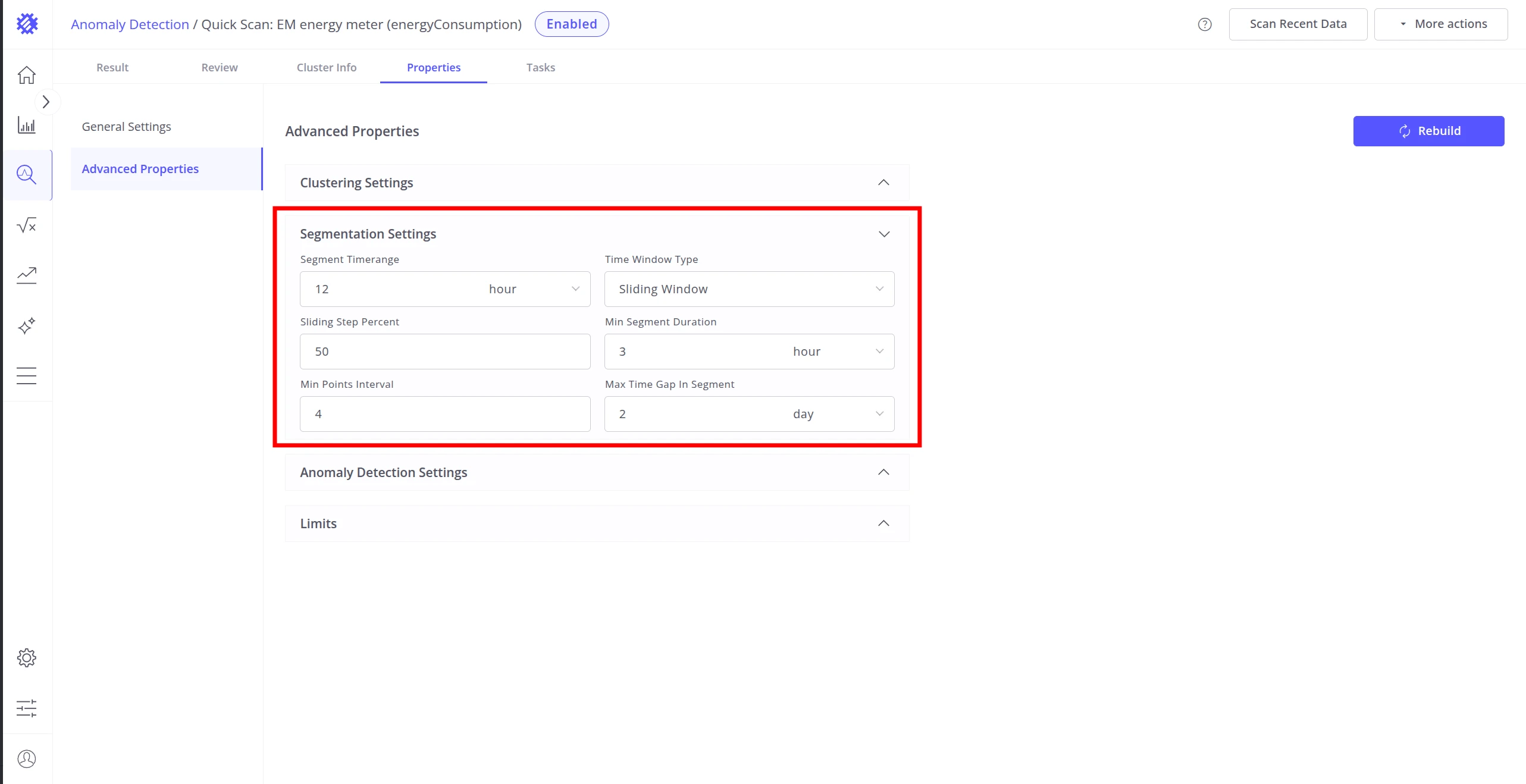
Segmentation Settings
Section titled “Segmentation Settings”Segmentation splits continuous telemetry into fixed-length time windows before clustering.
  Raw telemetry stream  ────────────────────────────────────────────────▶ time
  Fixed Range (non-overlapping):  ╔══════════╗ ╔══════════╗ ╔══════════╗  ║ segment1 ║ ║ segment2 ║ ║ segment3 ║  ╚══════════╝ ╚══════════╝ ╚══════════╝
  Sliding Window (overlapping, step = 50%):  ╔══════════╗  ║ segment1 ║  ╚══════════╝        ╔══════════╗        ║ segment2 ║        ╚══════════╝              ╔══════════╗              ║ segment3 ║              ╚══════════╝
▶ Sliding Window produces more segments than Fixed Range due to overlap — this increases training time and memory.| Setting | Description |
|---|---|
| Segment Time Range | Duration of each data window, e.g. 6 hours, 1 day. Match this to natural cycles of your system. |
| Time Window Type | Fixed Range — non-overlapping windows. Sliding Window — overlapping windows that advance by a fixed step. Sliding produces more segments, which increases training time and memory usage. |
| Sliding Step Percent | Step size as a percentage of the segment duration (Sliding Window only). |
| Max Time Gap in Segment | Maximum allowed gap between consecutive data points within a segment. Segments with larger gaps are discarded. |
| Min Segment Duration | Minimum elapsed time for a segment to be considered valid. |
| Min Points in Segment | Minimum number of data points required for a valid segment. |
Anomaly Detection Settings
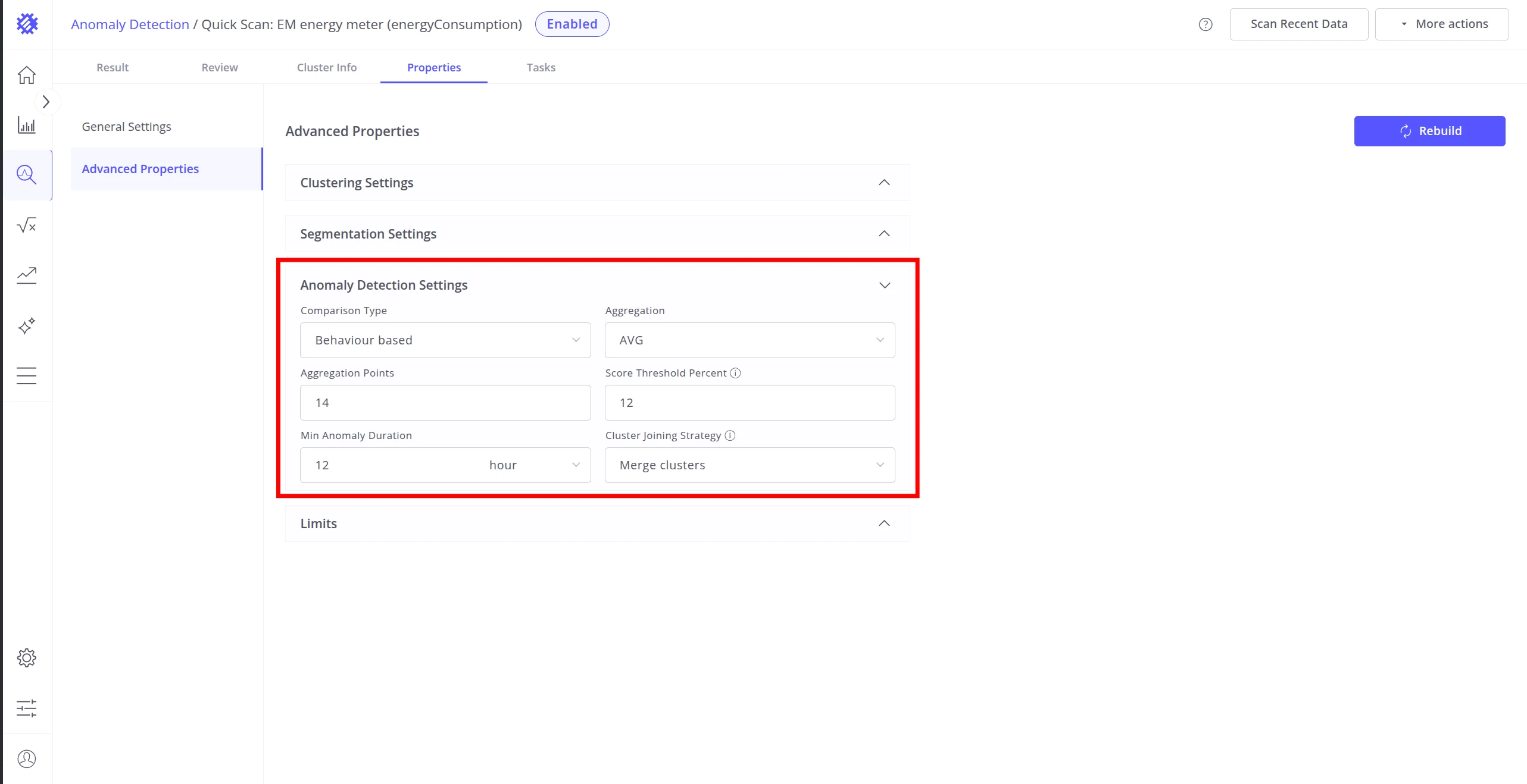
Section titled “Anomaly Detection Settings”After segmentation, each segment is scored for how much it deviates from normal clusters.
Comparison Type controls how segments are represented before comparison:
- Feature-based — extracts statistical attributes from each segment (mean, std, slope). Focuses on specific measurable properties of the data.
- Behavior-based — captures the overall shape and trend of the segment by aggregating it into a fixed number of points.
Behavior-based additional parameters:
| Setting | Description |
|---|---|
| Aggregation | Function used to summarize each sub-interval: AVG, MIN, MAX, SUM, or COUNT. |
| Aggregation Points | Number of sub-intervals each segment is divided into before aggregation. |
Scoring and filtering:
| Setting | Description |
|---|---|
| Score Threshold Percent | Percentile cutoff for classifying a segment as anomalous. For example, 15% means the top 15% of highest-scoring segments are marked as anomalies. |
| Min Anomaly Duration | Minimum duration an anomalous event must last to be reported. Filters out very short noise spikes. |
| Cluster Joining Strategy | When enabled, treats anomalies from consecutive segments — even across different clusters — as a single continuous anomaly. Two anomalous segments are joined when the gap between them does not exceed the Max Time Gap in Segment threshold. |
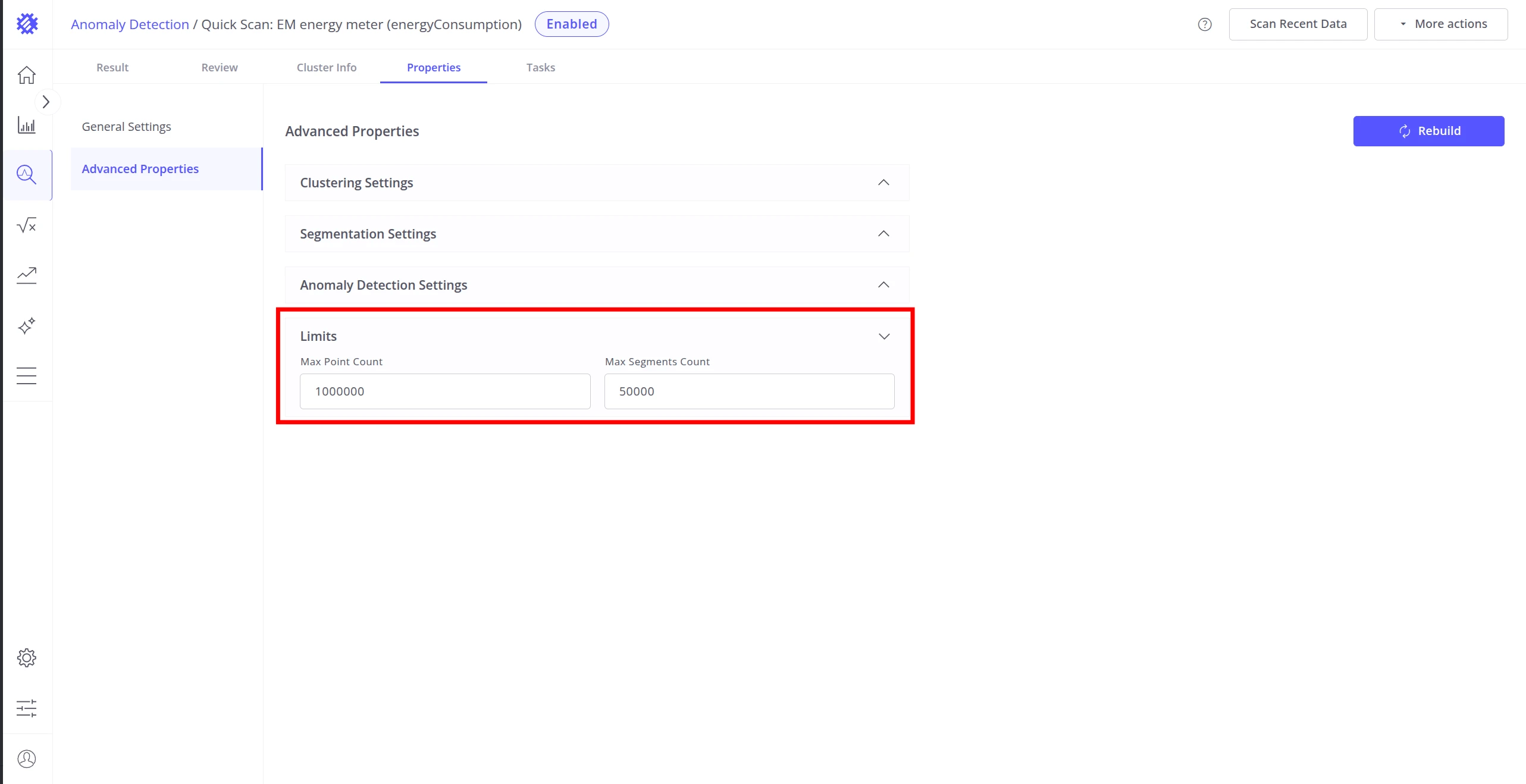
Limits
Section titled “Limits”Limits cap the volume of data processed during training and detection. When a limit is reached, the data is truncated to the specified count — training continues with the available subset. Set limits conservatively on large datasets to avoid long training times.
| Setting | Description |
|---|---|
| Max Points Count | Maximum number of individual telemetry data points used for training. Excess points are truncated. |
| Max Segments Count | Maximum number of segments the model will process. Excess segments are truncated. |
Building the Model
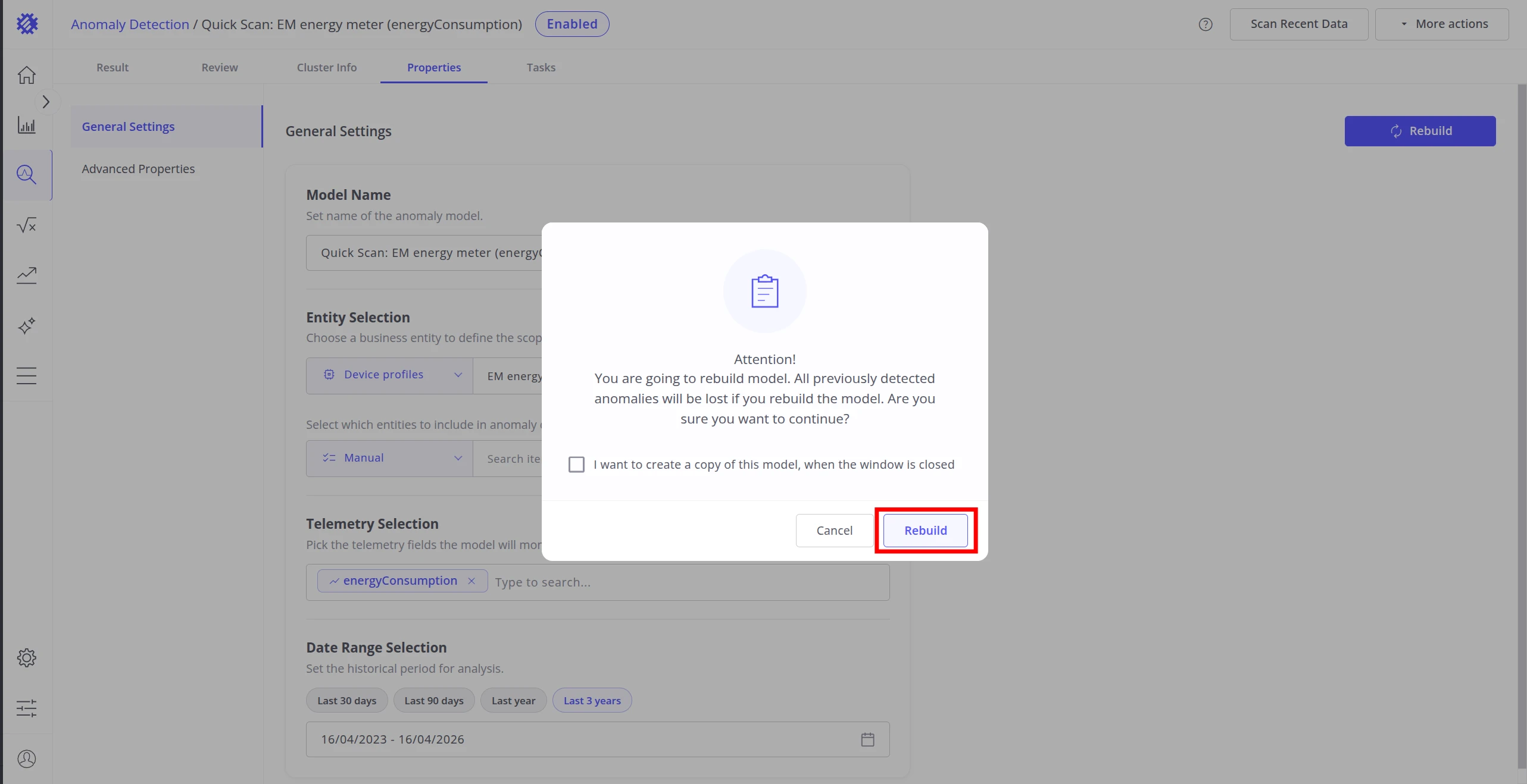
Section titled “Building the Model”Once all properties are configured, use the Build model button in the top right to train the model for the first time. The button is labeled Rebuild on models that have already been built at least once.
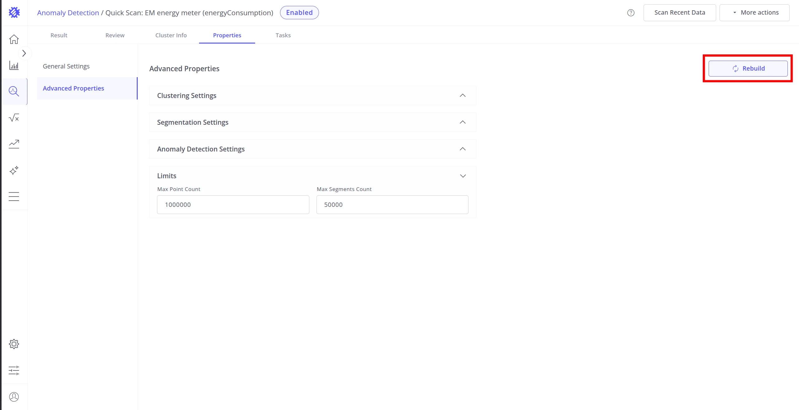
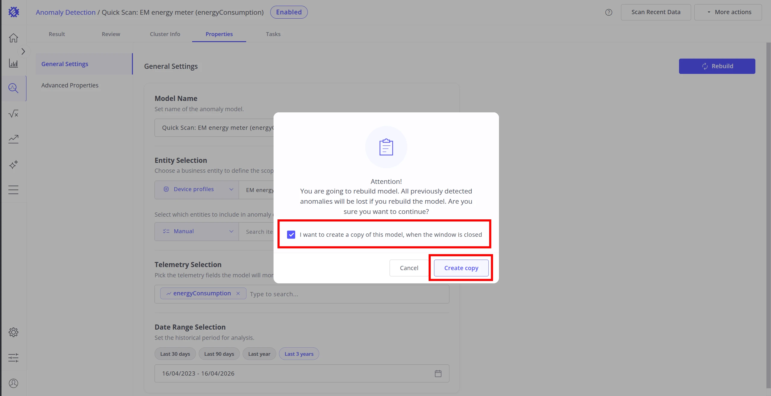
Clicking Rebuild opens a confirmation dialog. Rebuilding retrains the model from scratch — all previously detected anomalies are lost. Optionally, check I want to create a copy of this model to preserve the current configuration as a new model before rebuilding starts.
Best Practices
Section titled “Best Practices”| Area | Recommendation |
|---|---|
| Training data | Use data that represents normal behavior. Build on all devices first to identify the most representative ones, then retrain on those. |
| Segmentation | Match segment duration to natural cycles of your system (e.g. shift length, maintenance intervals). |
| Clustering algorithm | Use DBSCAN for noisy or irregularly shaped data; K-Means for clean, well-separated clusters; GMM when cluster boundaries overlap. |
| Score threshold | Start with a higher threshold (fewer anomalies) and lower it gradually as you validate results. |
| Performance | Set Limits conservatively on large datasets to avoid long training times. |
Was this helpful?