Forecasting Methods & Accuracy (Prophet, ARIMA)
This page describes a prediction model after you build it: how it stays up to date, the settings on its Properties tab, the methods it can learn with, and how accurate it is. Trendz trains the model separately for every item of the profile, so ten meters get ten models, each learning its own history.
To build your first model, start with Getting started.
| Section | What it covers |
|---|---|
| Model lifecycle | How the model is trained, and how it keeps up with new readings |
| Properties tab | Every setting of the model, and how to change it |
| Wizard advanced settings | The method and forecast limits, set before the build |
| Prediction methods | The built-in algorithms, and how to write your own in Python |
| Accuracy | How close the forecasts come to what really happened |
Model lifecycle
Section titled “Model lifecycle”A model works in two kinds of runs. Training learns the patterns of each item from its history. Refresh reads the newest readings, predicts again with the trained model, and sends the forecast and alarms to ThingsBoard.
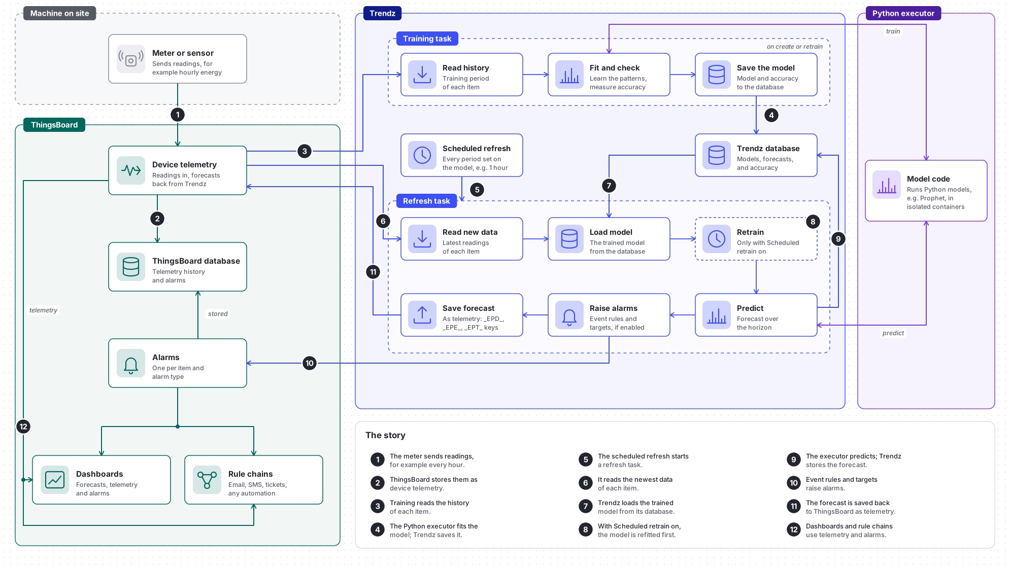
| Run | Started by |
|---|---|
| Training (steps 3–4) | Build model in the wizard, Rebuild after Apply changes on the Properties tab, Retrain in an item’s row menu, or Retrain all failed on the Data status card |
| Refresh (steps 5–11) | Periodic refresh on its schedule, set in Monitoring & Alarms, Refresh in an item’s row menu, or Refresh item and Refresh all on the Data status card |
Properties tab
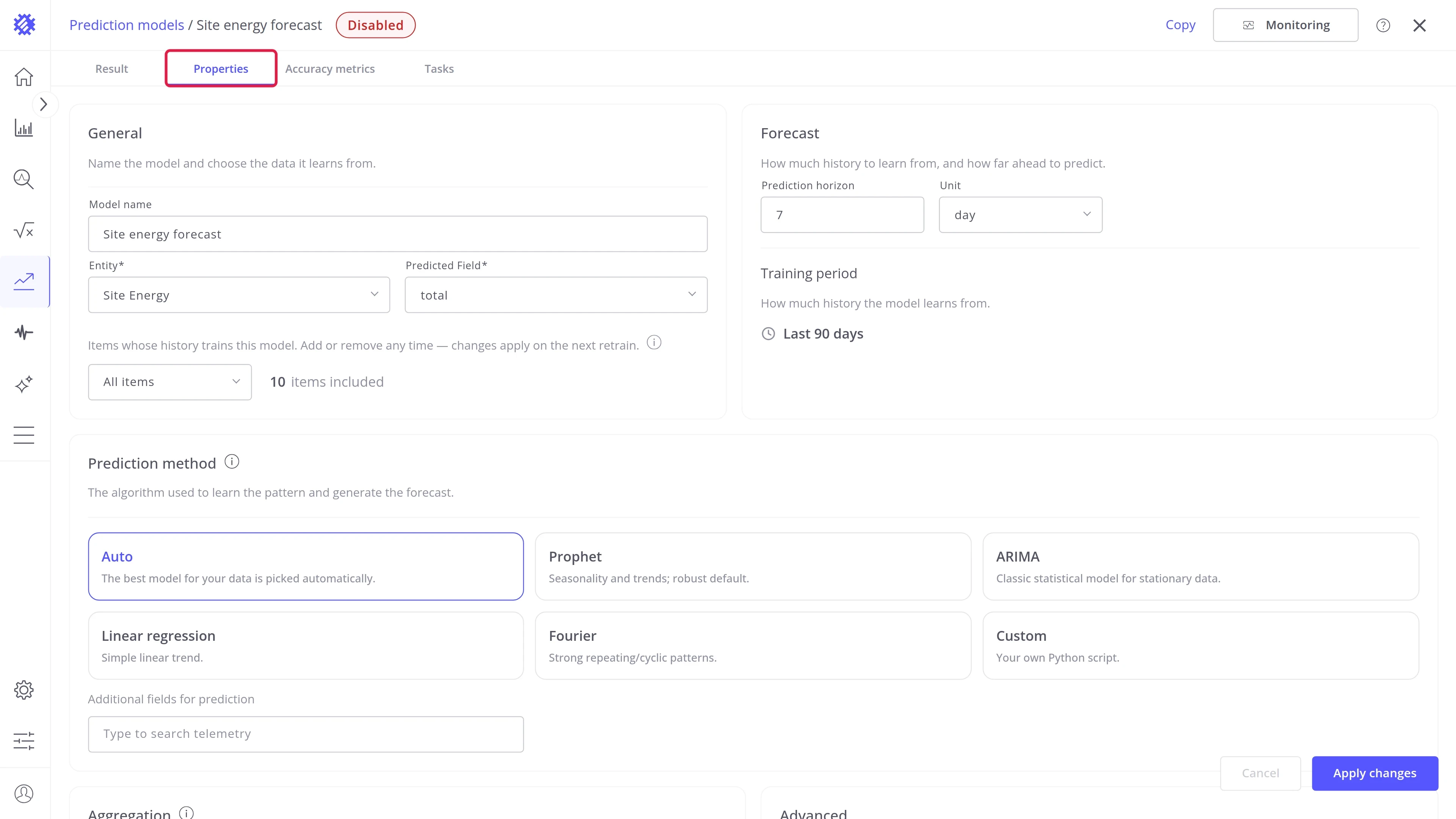
Section titled “Properties tab”The Properties tab shows how the model is set up. Here you can check its settings and change them when needed: the data it learns from, how far ahead it predicts, and how it learns.
To open it, click Properties in the tabs of the model page.
Layout
Section titled “Layout”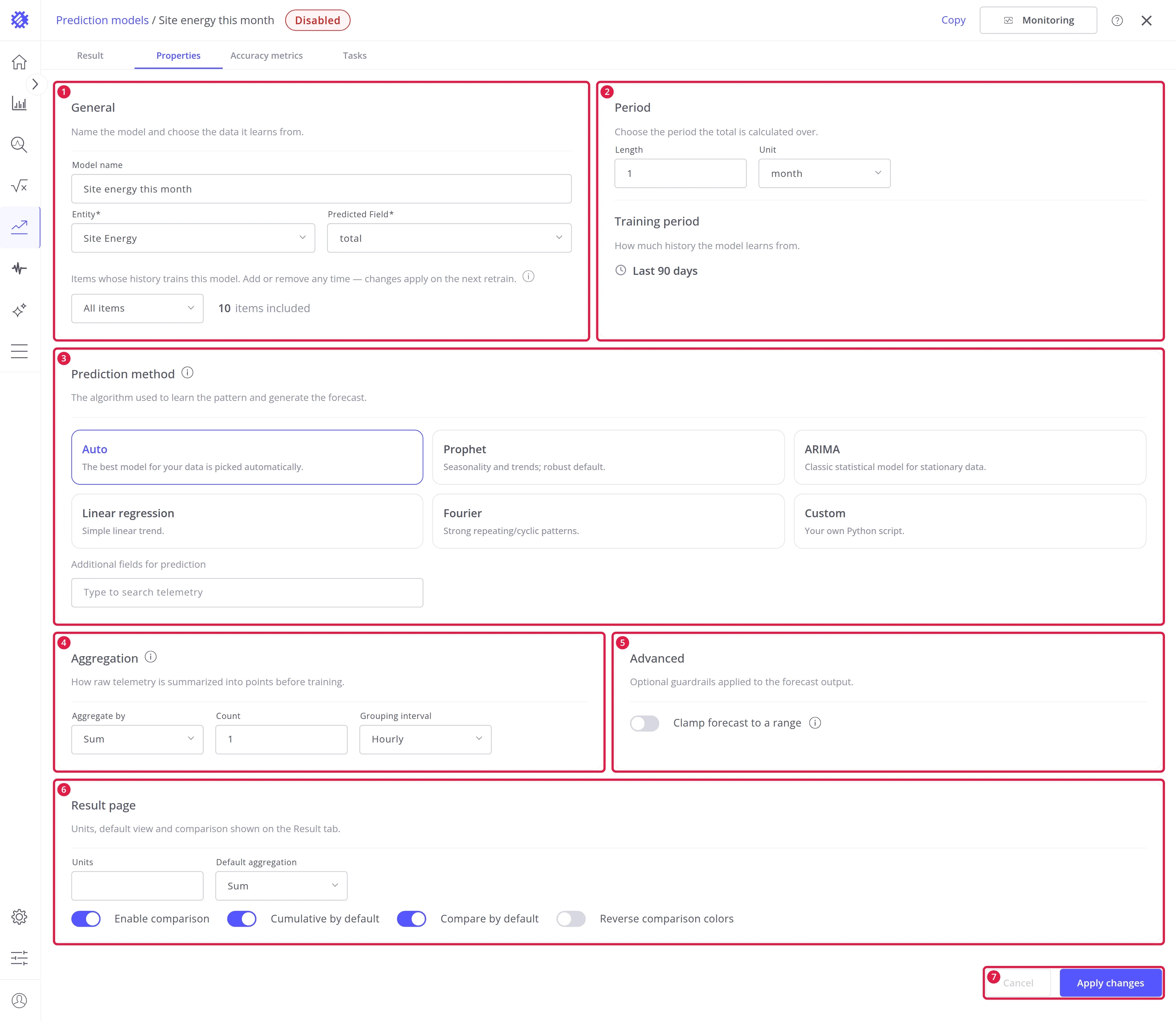
| # | Area | Contents |
|---|---|---|
| 1 | General | The model name, the profile, the predicted field, and which items to train |
| 2 | Forecast or Period | How far ahead to predict, or the period to predict over, and how much history to learn from |
| 3 | Prediction method | The algorithm, and other fields that help it |
| 4 | Aggregation | How the readings become one point per interval |
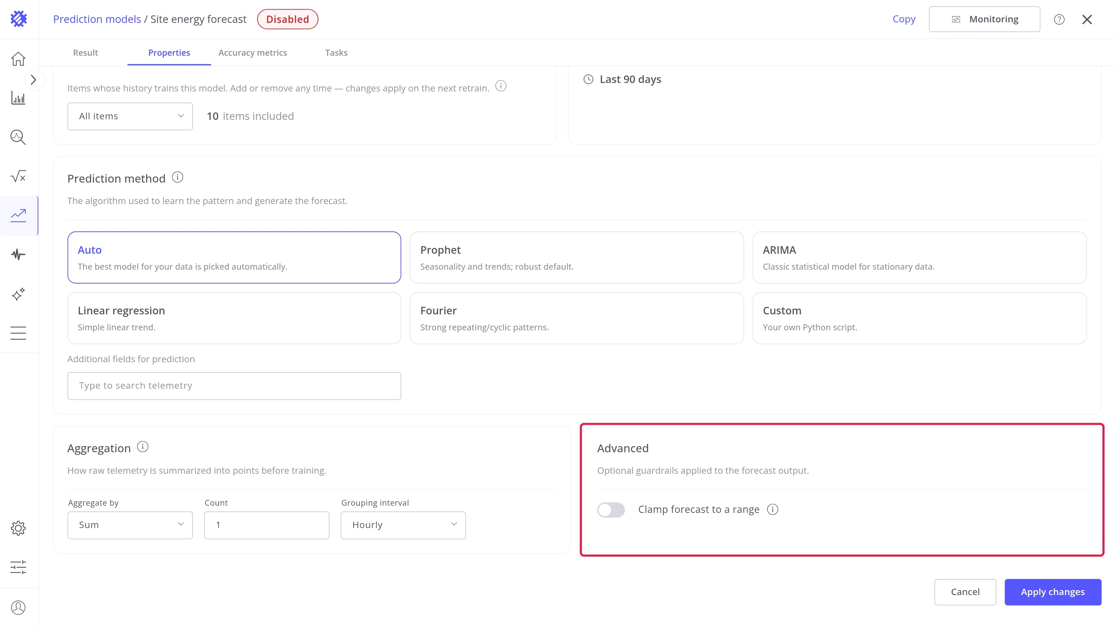
| 5 | Advanced | Limits for the forecast |
| 6 | Result page | How the Result tab opens. Time to Threshold, Period Total, and Hit Target only; described on Period Total |
| 7 | Cancel and Apply changes | Discard or apply the edits |
General
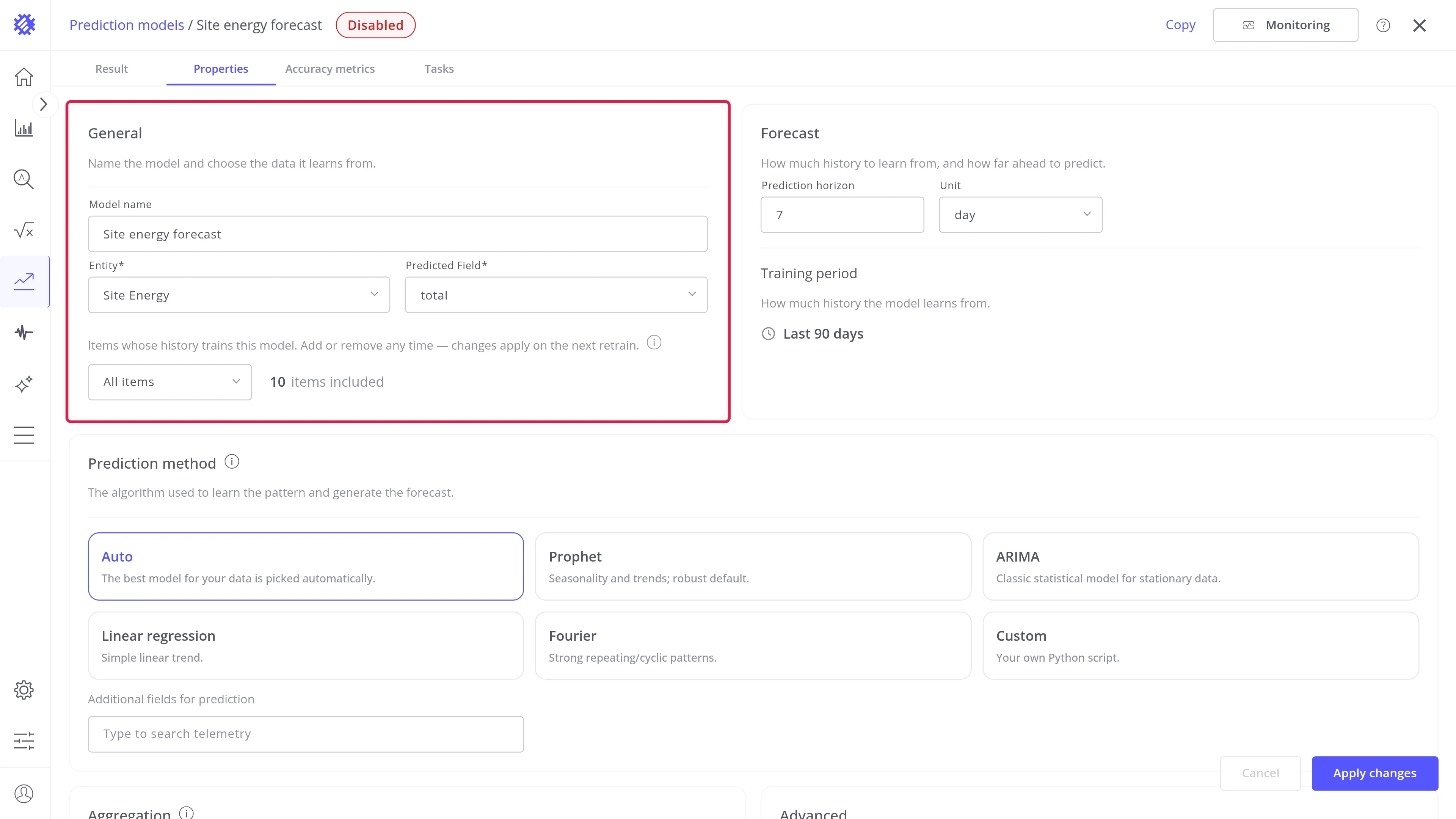
Section titled “General”The name of the model and the data it learns from.
| Field | Description |
|---|---|
| Model name | The name the model is listed under |
| Entity | The device or asset profile the model learns from |
| Predicted field | The telemetry key to predict |
| Items to train | All items: every item of the profile, including ones added later. Manual selection: only the items you pick |
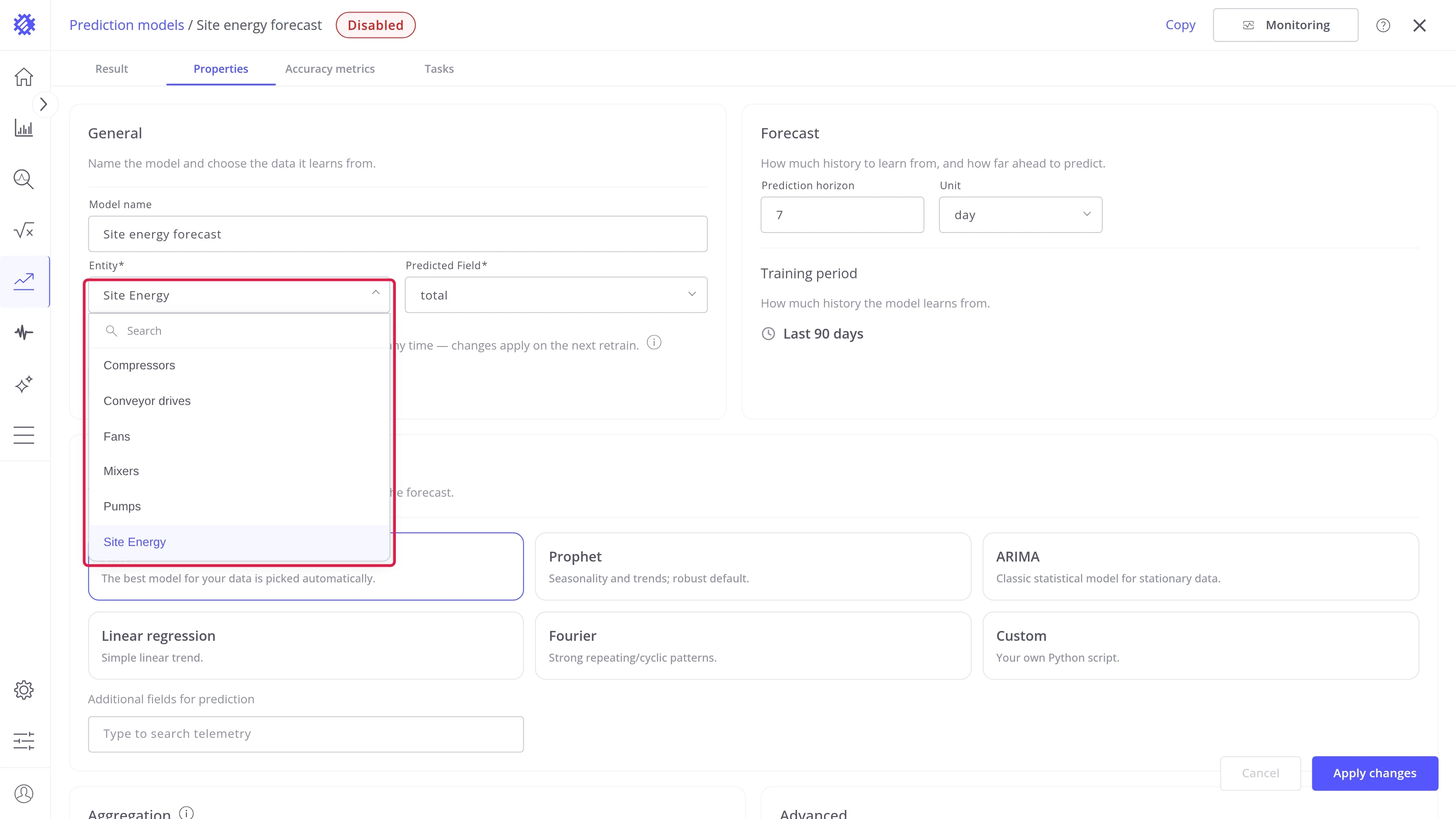
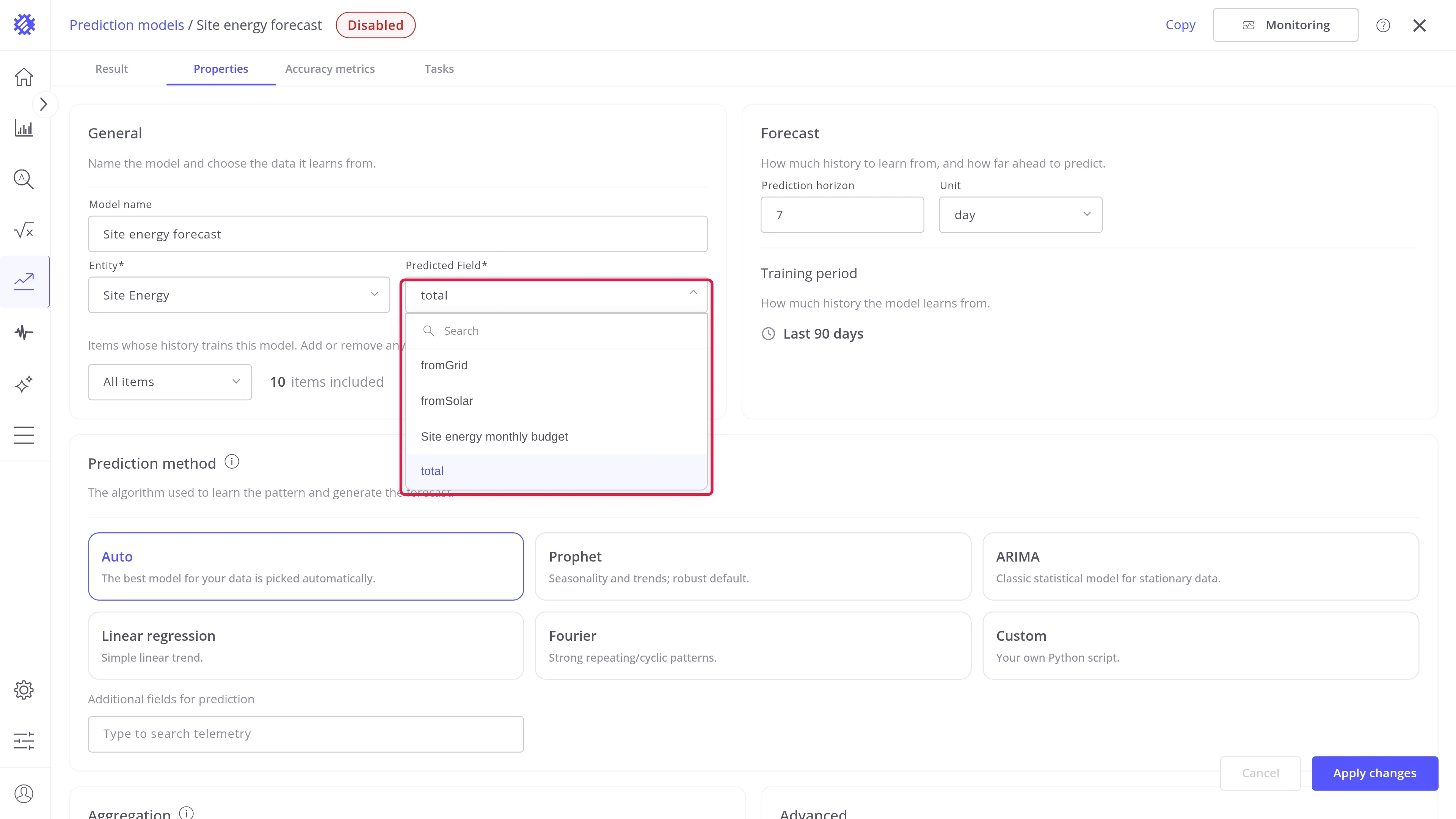
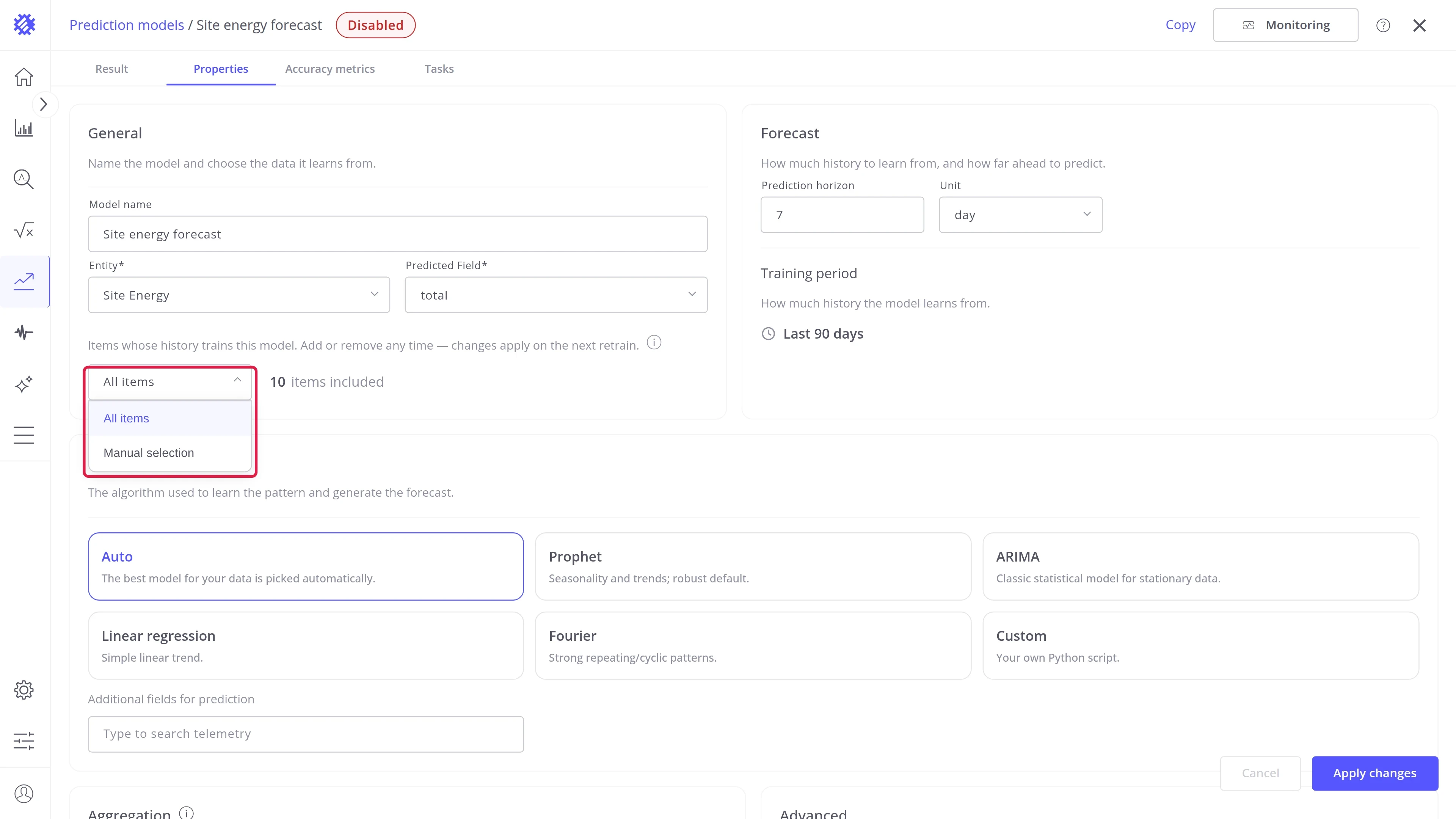
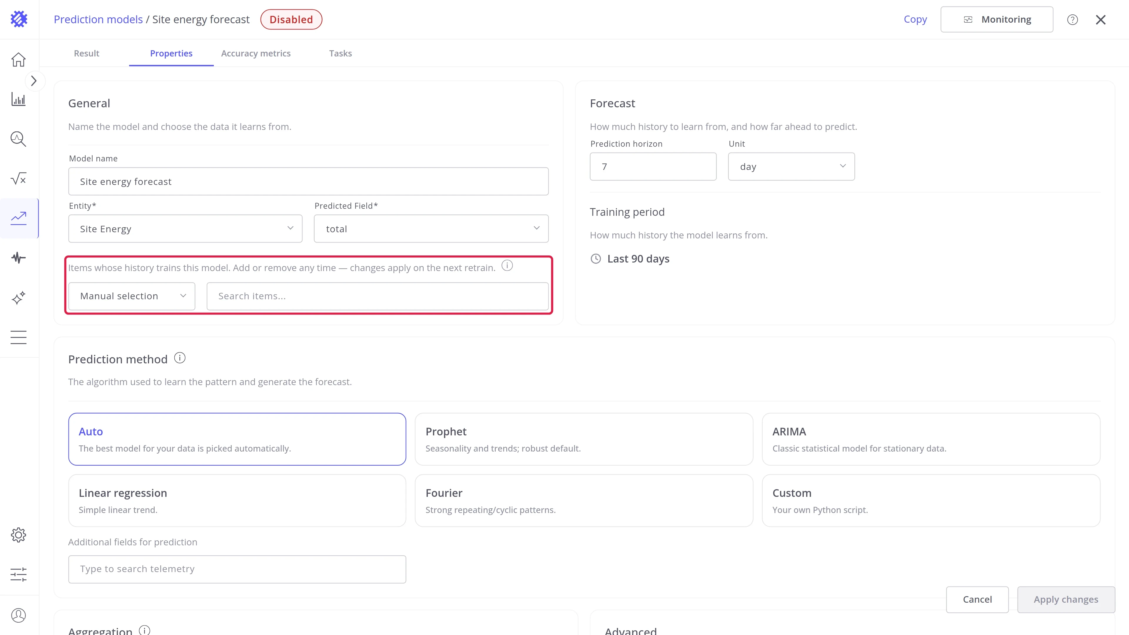
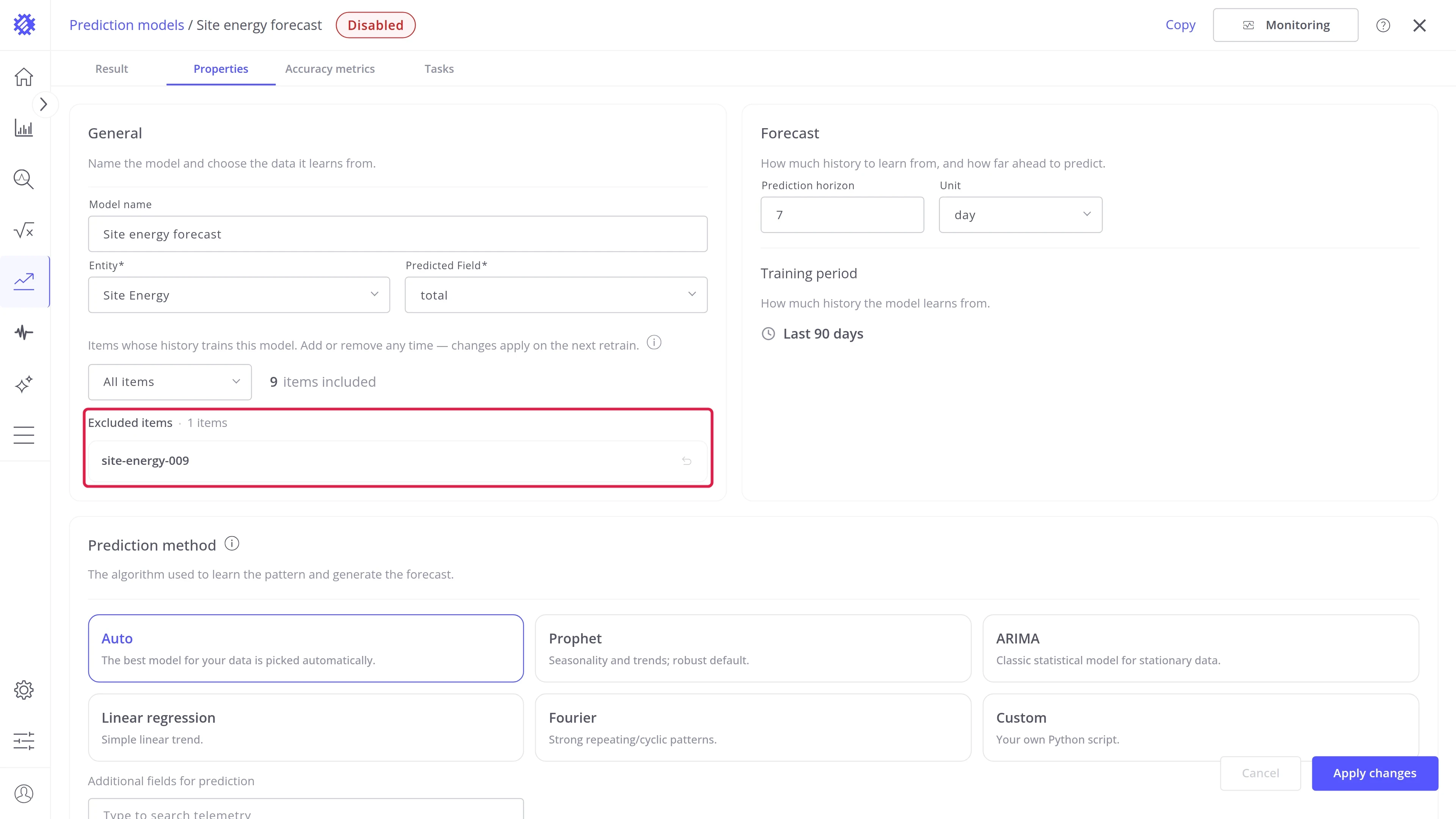
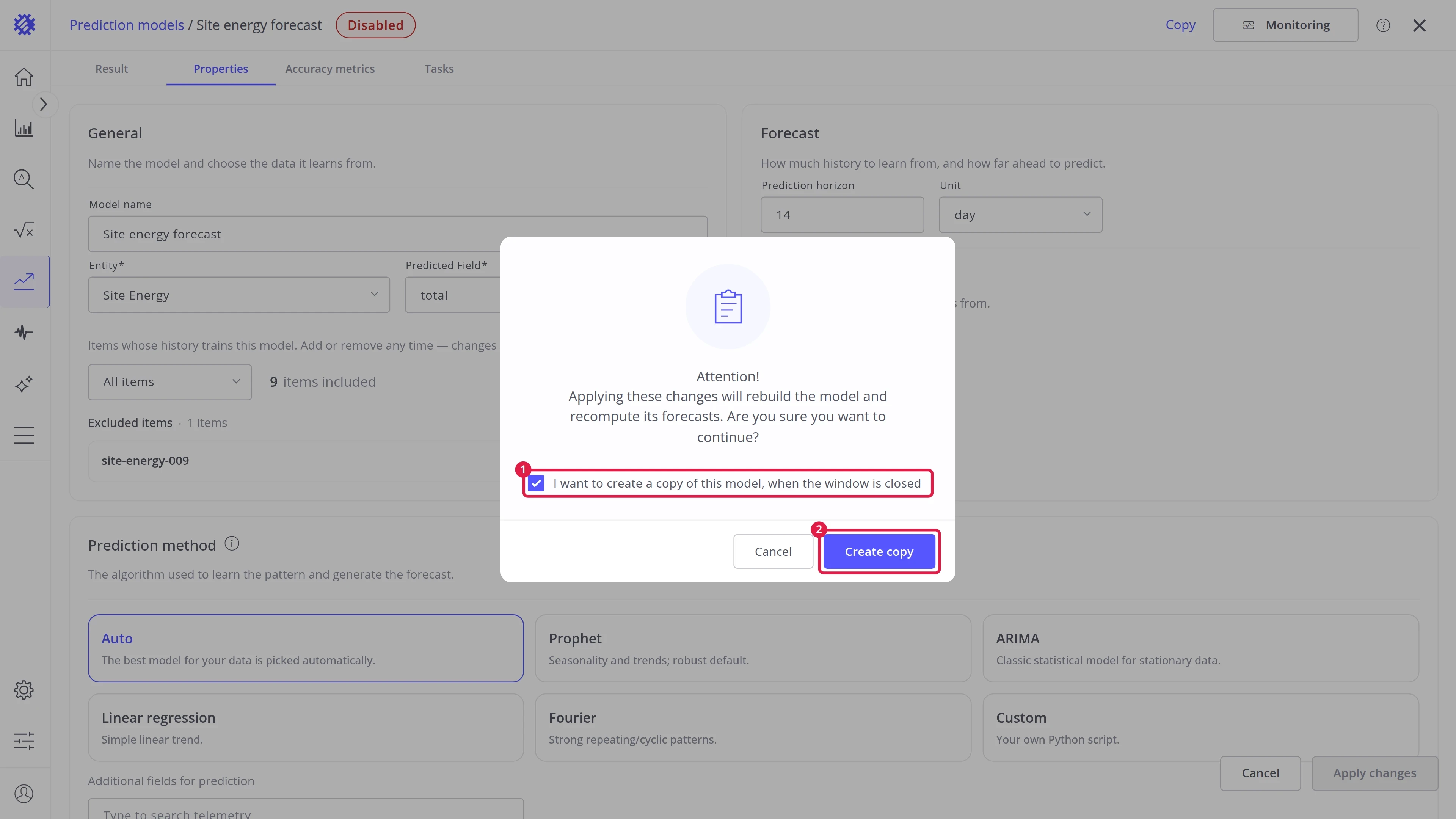
Excluded items. In All items mode, an item you delete from the model, with Delete in its row menu on the Result tab, is not trained or refreshed any more and is listed under Excluded items. Its history stays in ThingsBoard. To bring it back:
- Open the Properties tab. The item is listed under Excluded items.
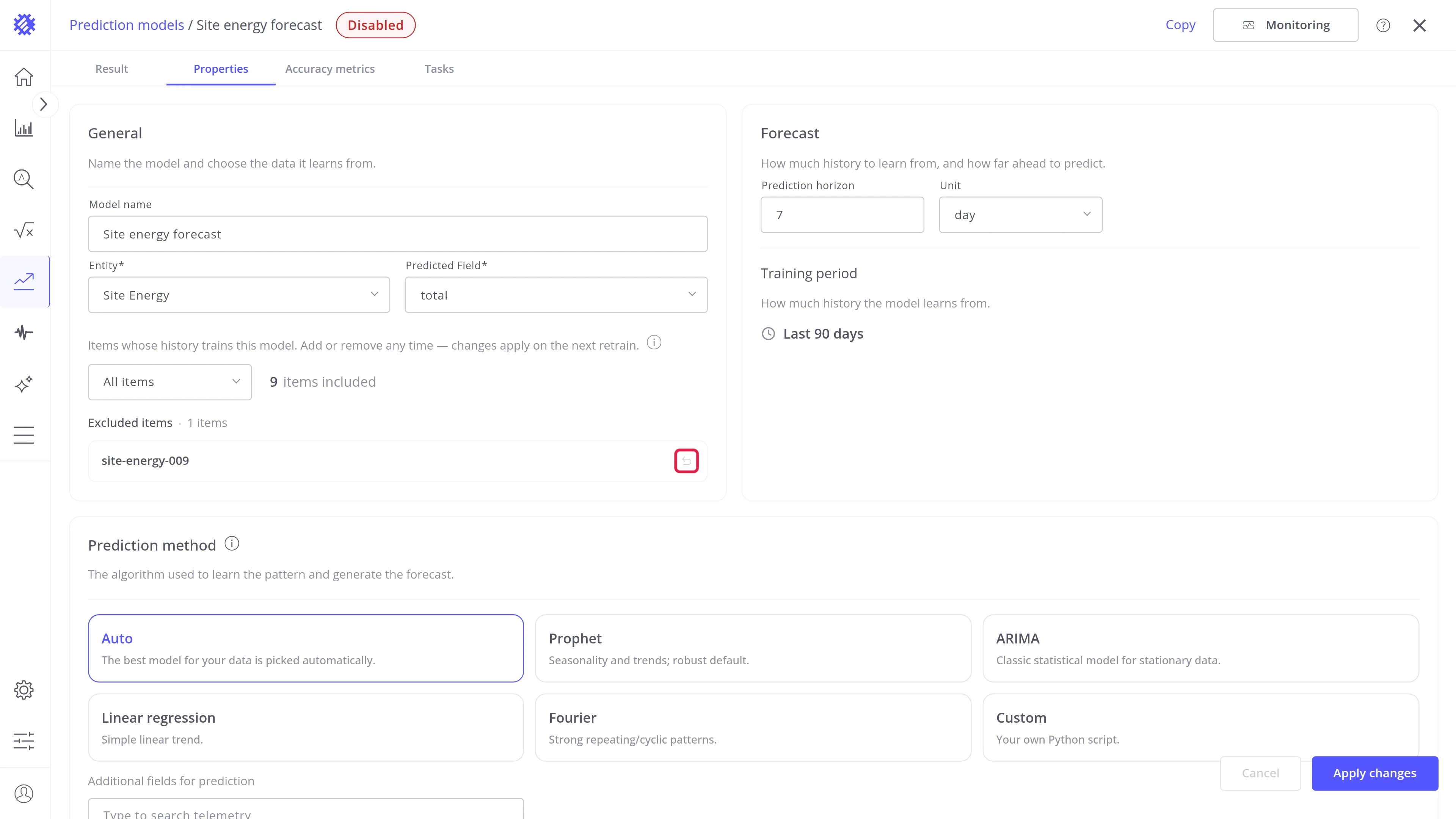
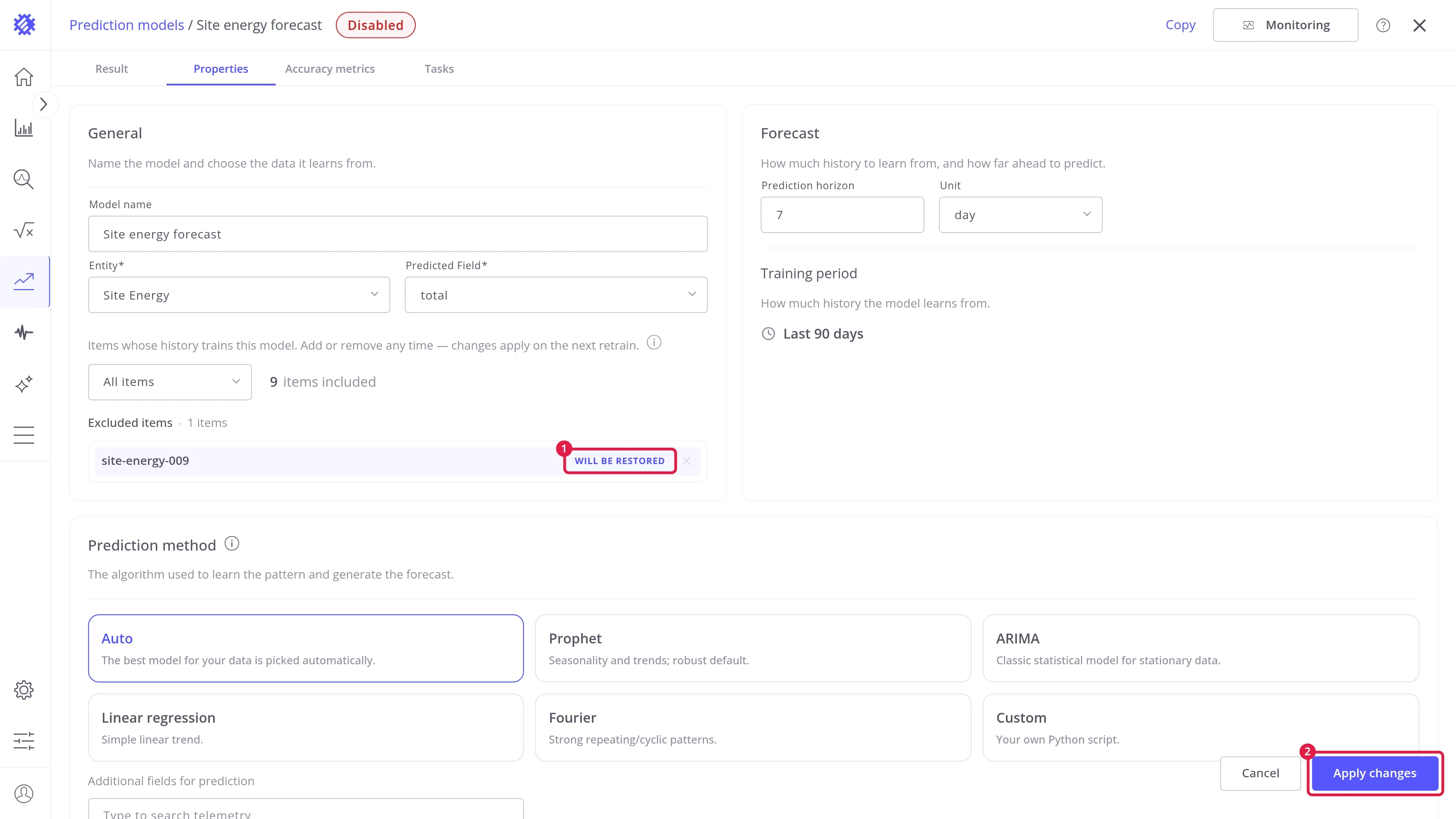
- Click the restore icon at the end of its row. It is marked Will be restored (1).
- Click Apply changes (2). The item returns to the model with the next training run.
Forecast
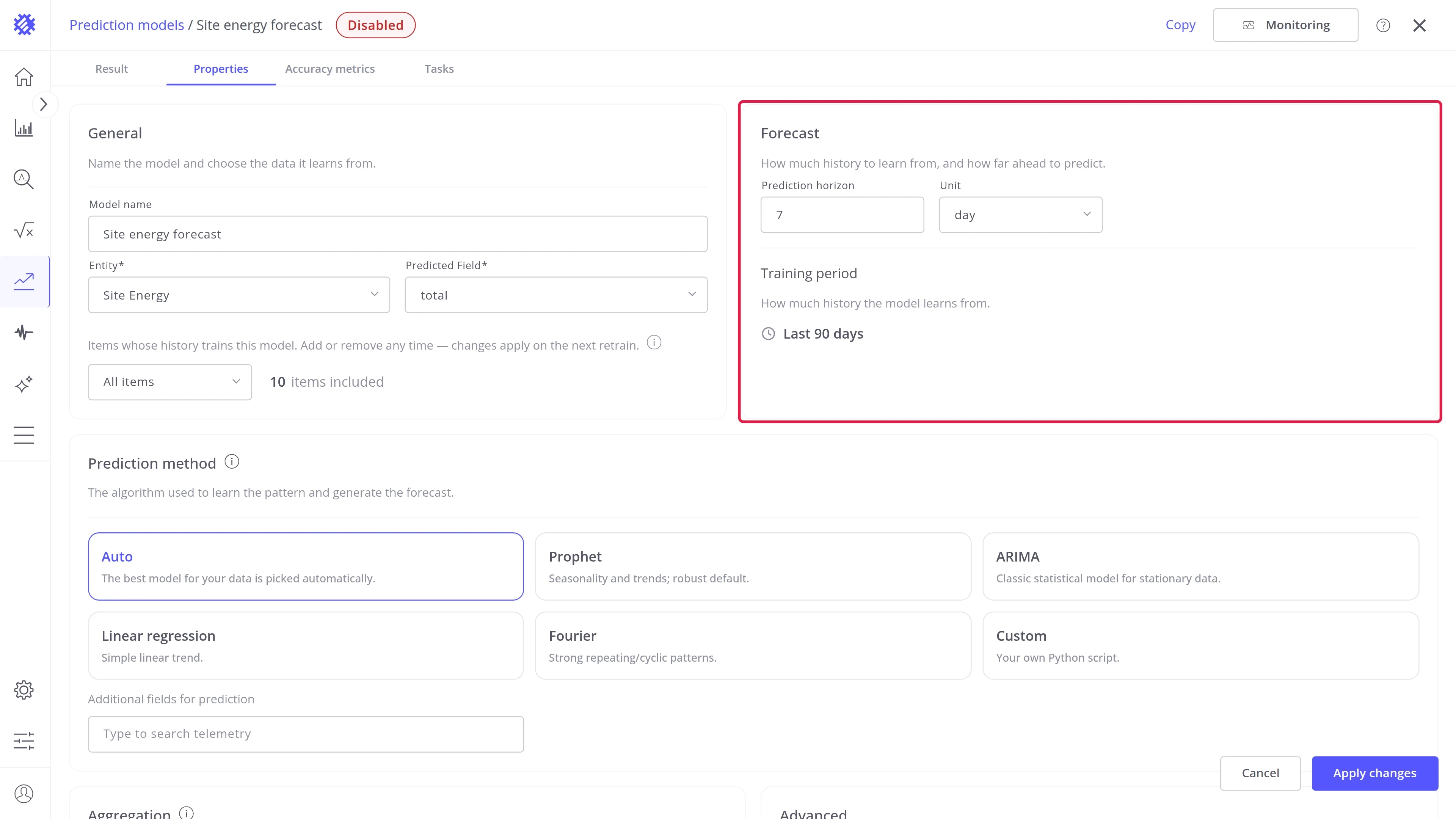
Section titled “Forecast”How far ahead the model predicts, and how much history it learns from.
| Field | Description |
|---|---|
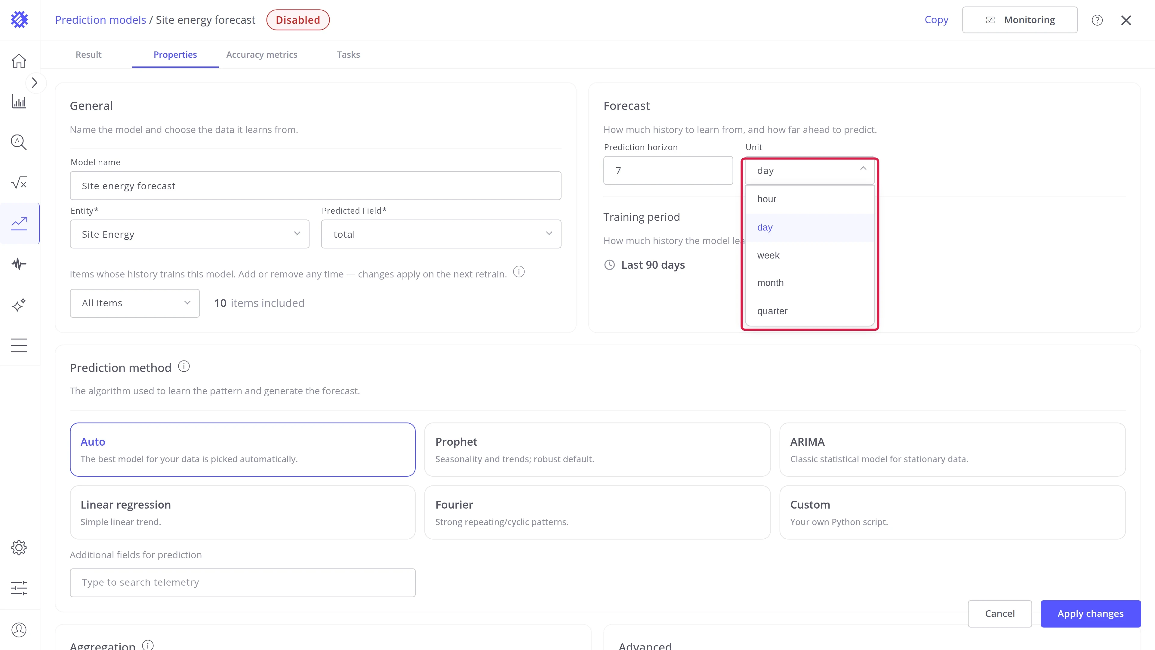
| Prediction horizon and Unit | How far ahead to predict, for example 7 days. The unit is hour, day, week, month, or quarter |
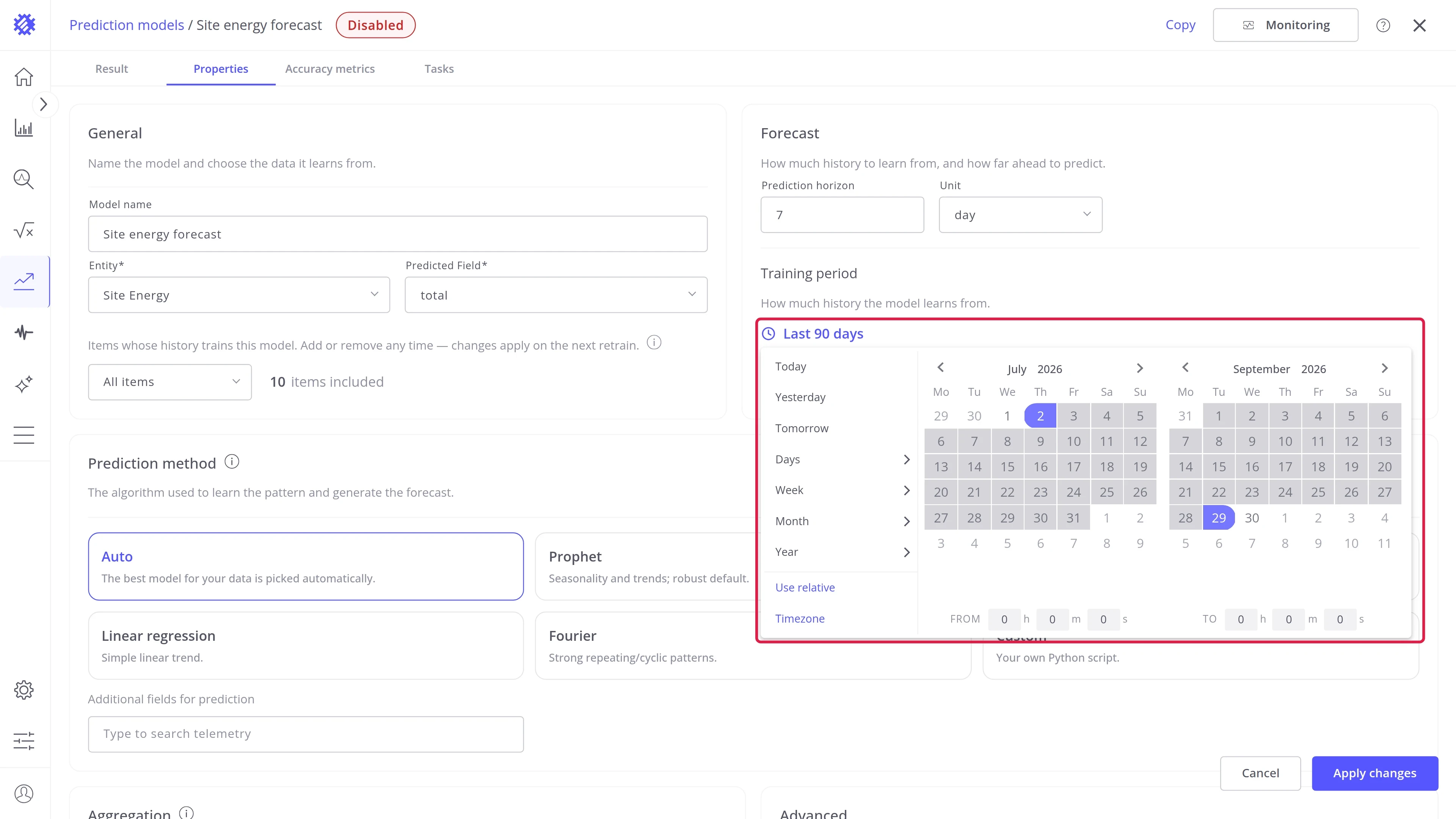
| Training period | How much history to learn from, for example the last 90 days |
Prediction method
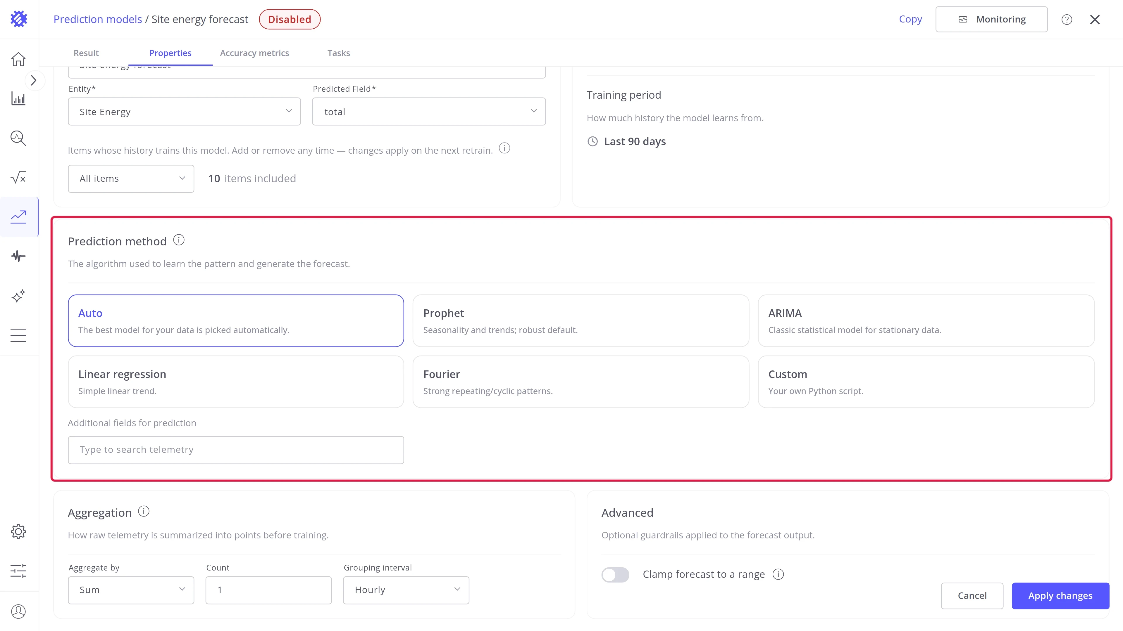
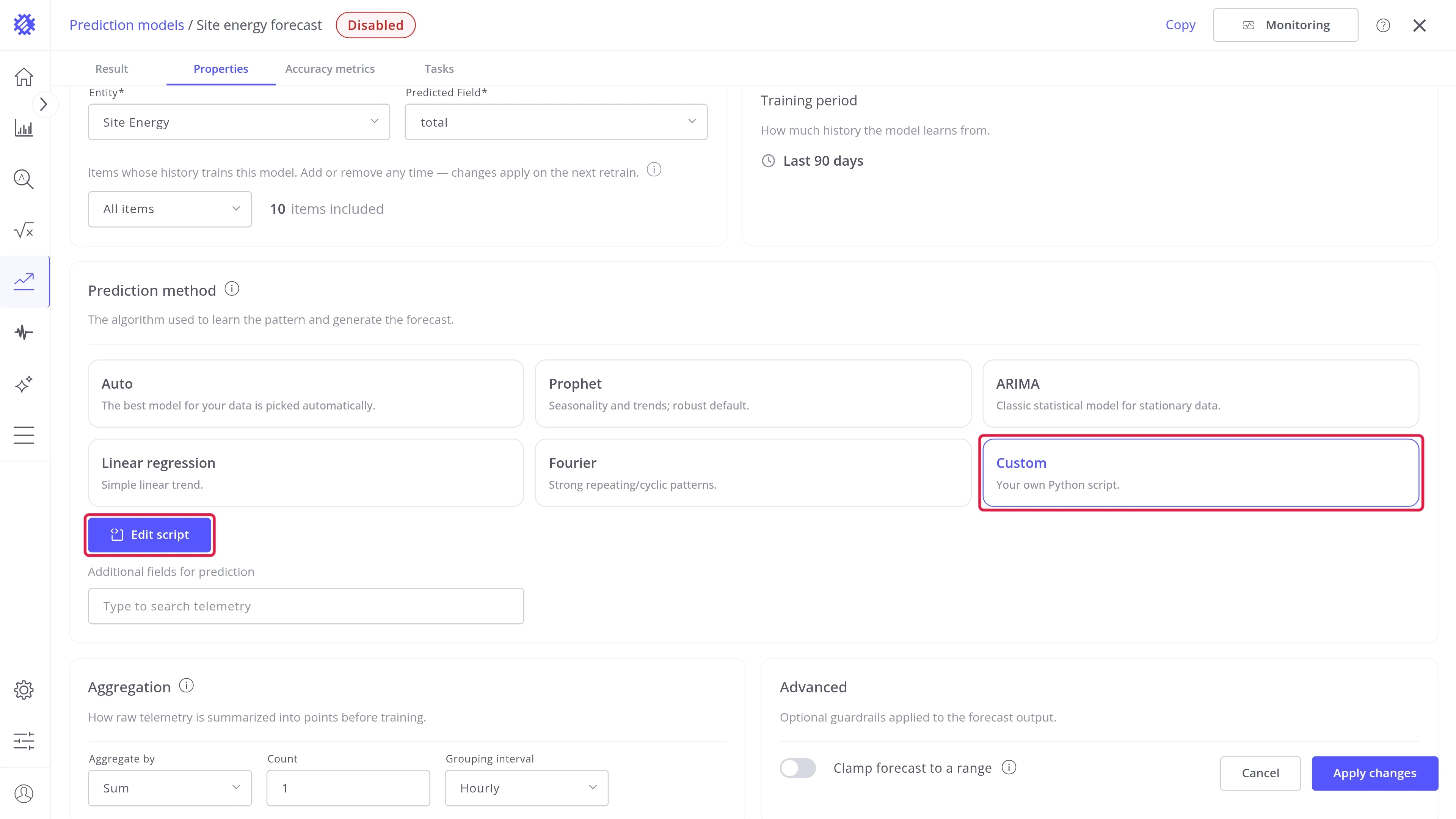
Section titled “Prediction method”The algorithm that learns from the history. Auto fits most data. Each method is described in Prediction methods.
| Field | Description |
|---|---|
| Method | Auto, Prophet, ARIMA, Linear regression, Fourier, or Custom |
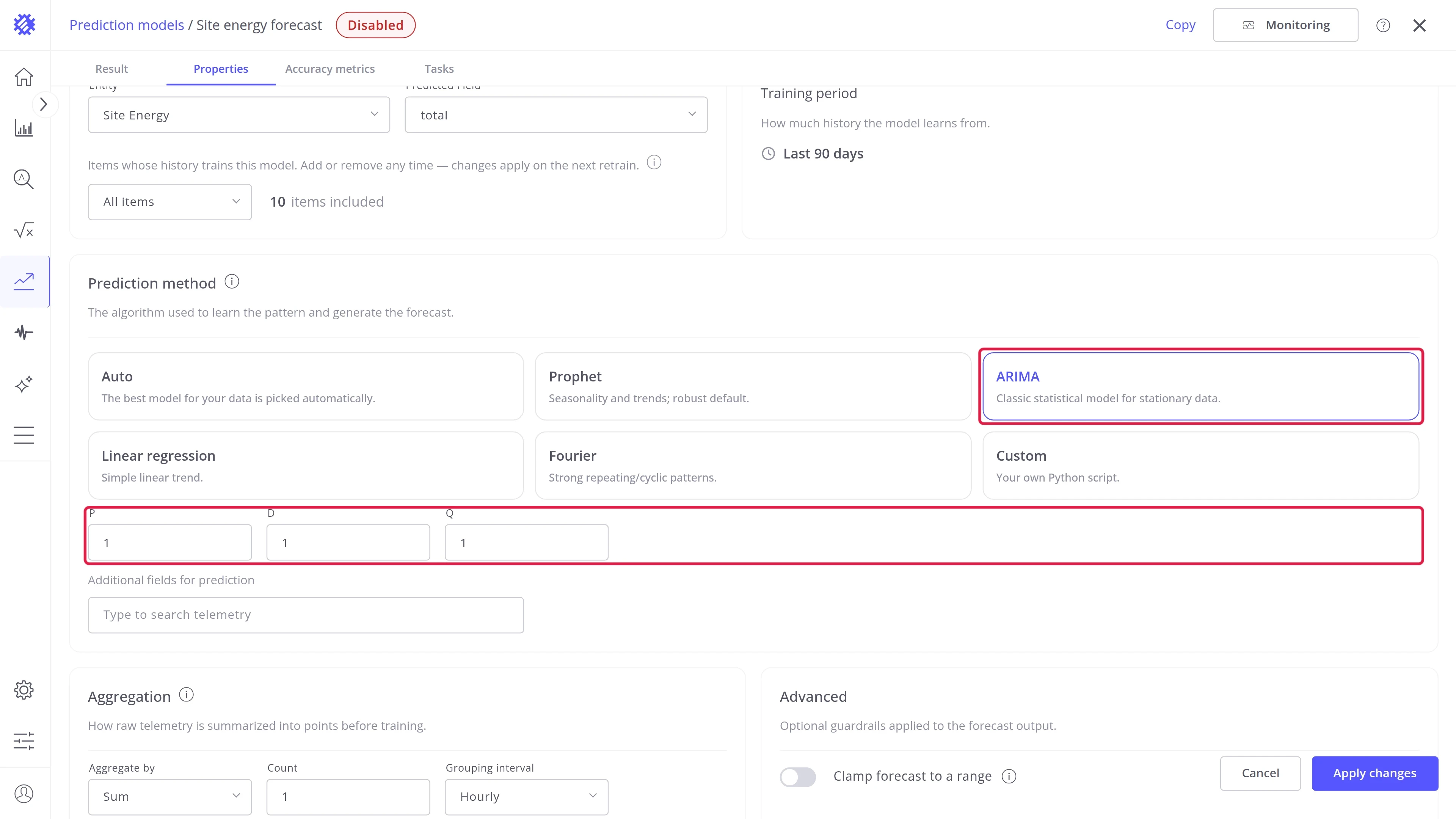
| P, D, Q | Shown for ARIMA: its autoregressive, differencing, and moving-average orders |
| Edit script | Shown for Custom: opens the Python editor, described in Custom models |
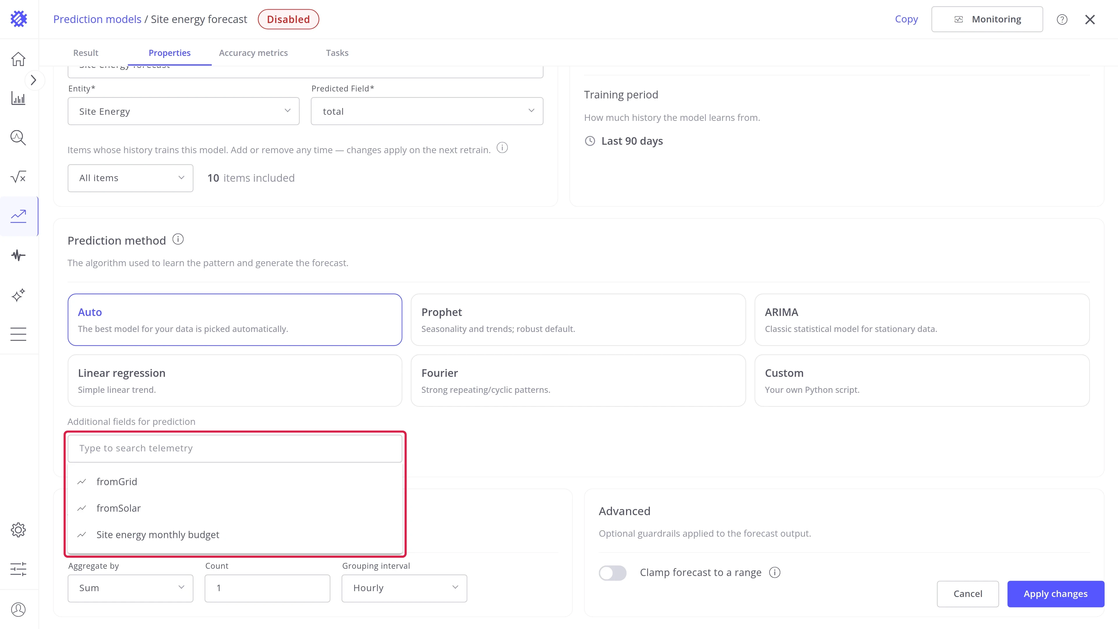
| Additional fields for prediction | Other telemetry of the same items that helps explain the predicted field, for example outdoor temperature for heating energy |
Aggregation
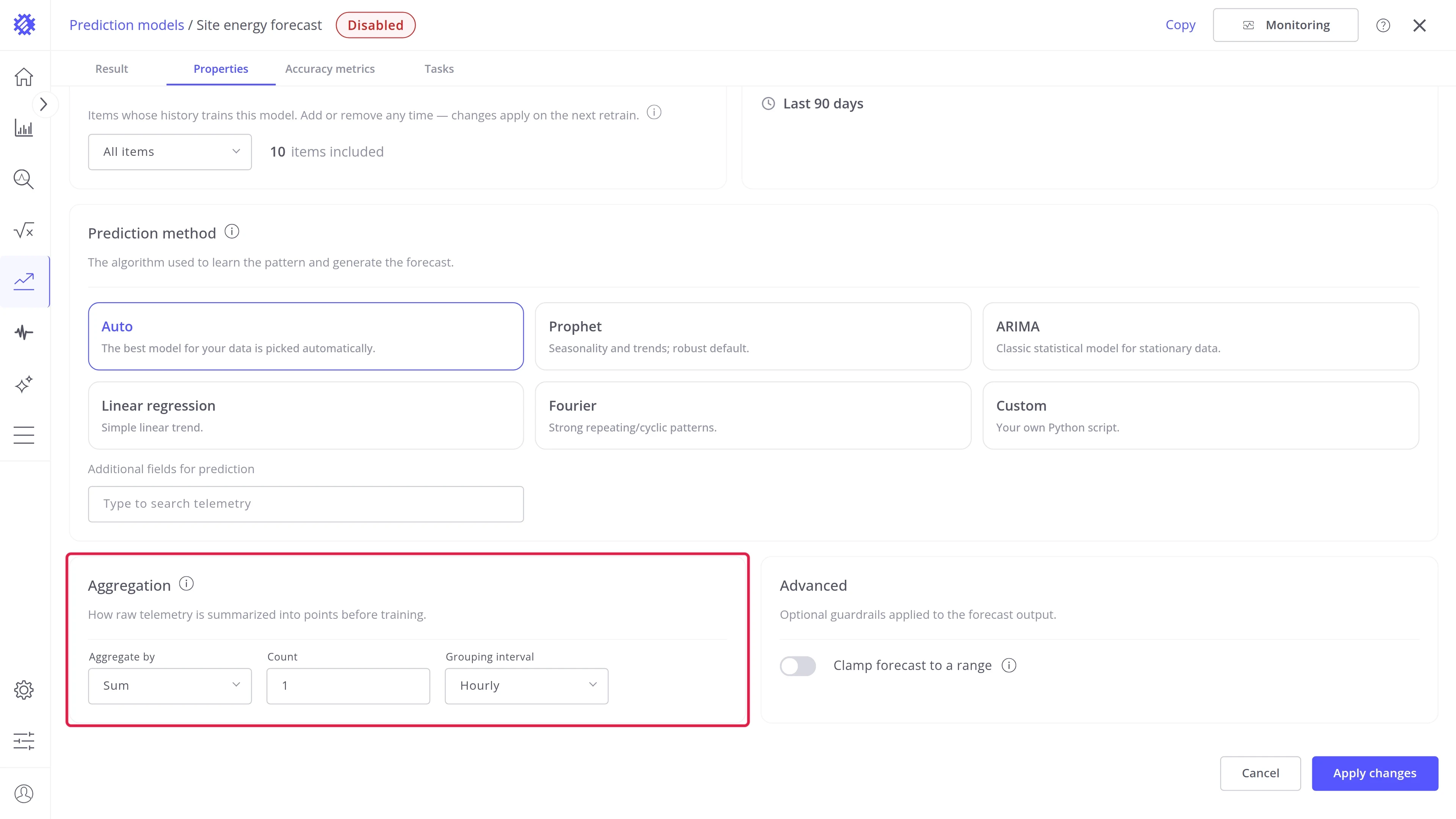
Section titled “Aggregation”How the raw readings are summarized into one point per interval before training. The forecast has the same step.
| Field | Description |
|---|---|
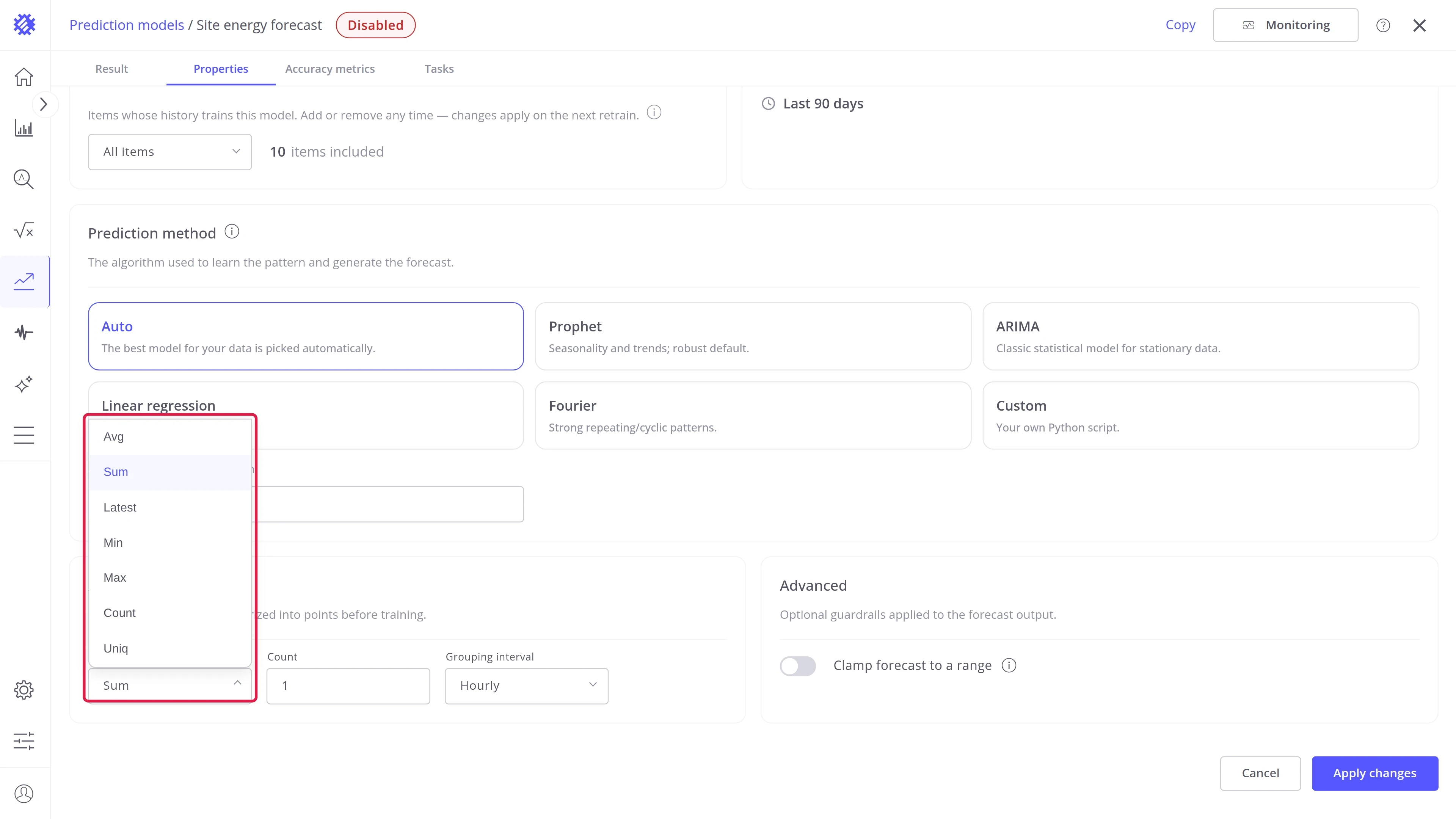
| Aggregate by | How the readings of one interval become one point: Avg, Sum, Latest, Min, Max, Count, or Uniq |
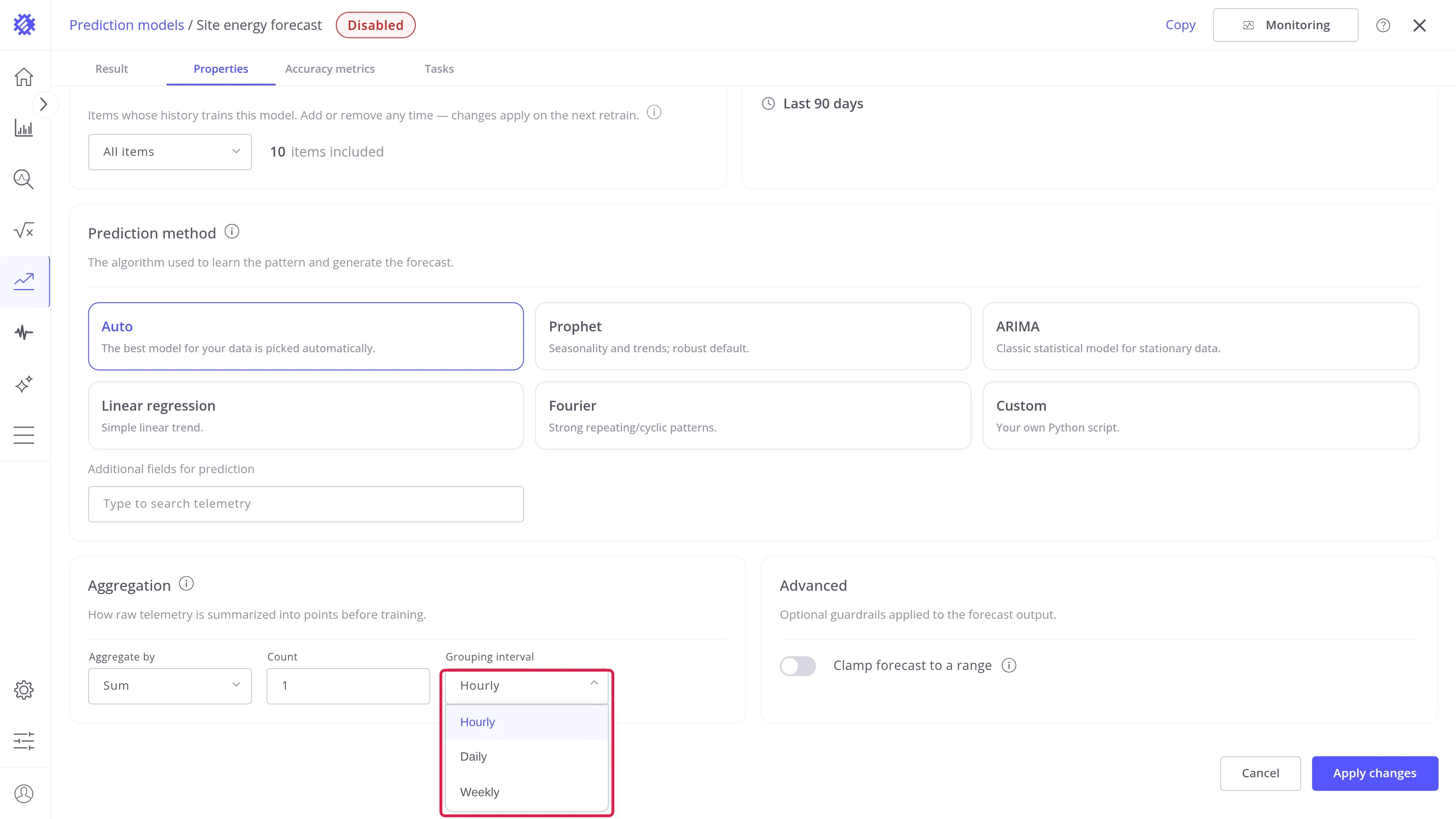
| Count and Grouping interval | The length of the interval: a count of Hourly, Daily, or Weekly units, for example 1 hour |
Advanced
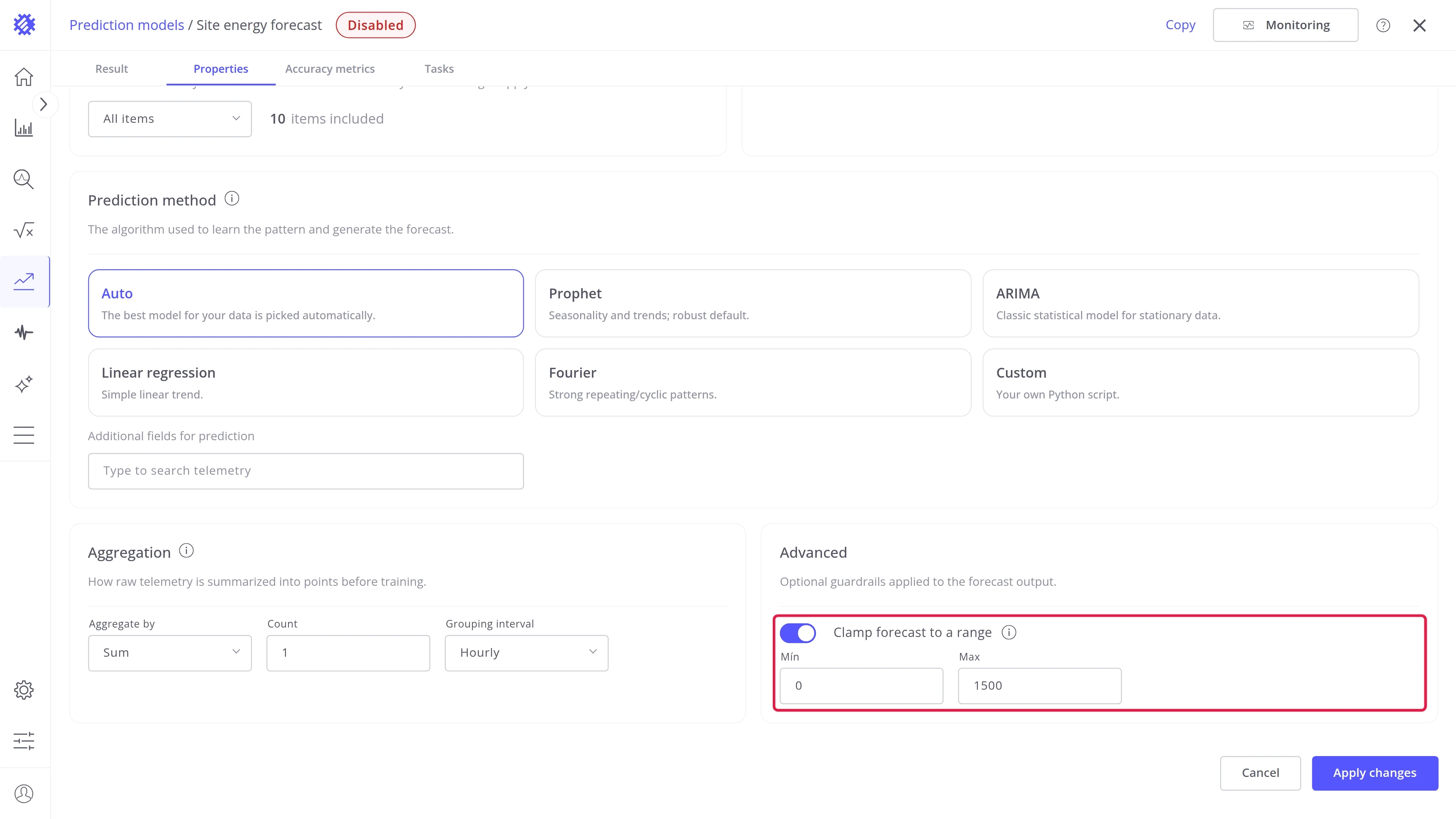
Section titled “Advanced”Limits for the forecast. Switch Clamp forecast to a range on and enter Min, Max, or both: predicted values below Min are raised to it, and values above Max are lowered to it. An empty field means no limit on that side. Use it for values that cannot leave a range, for example a tank level that cannot go below 0.
Applying changes
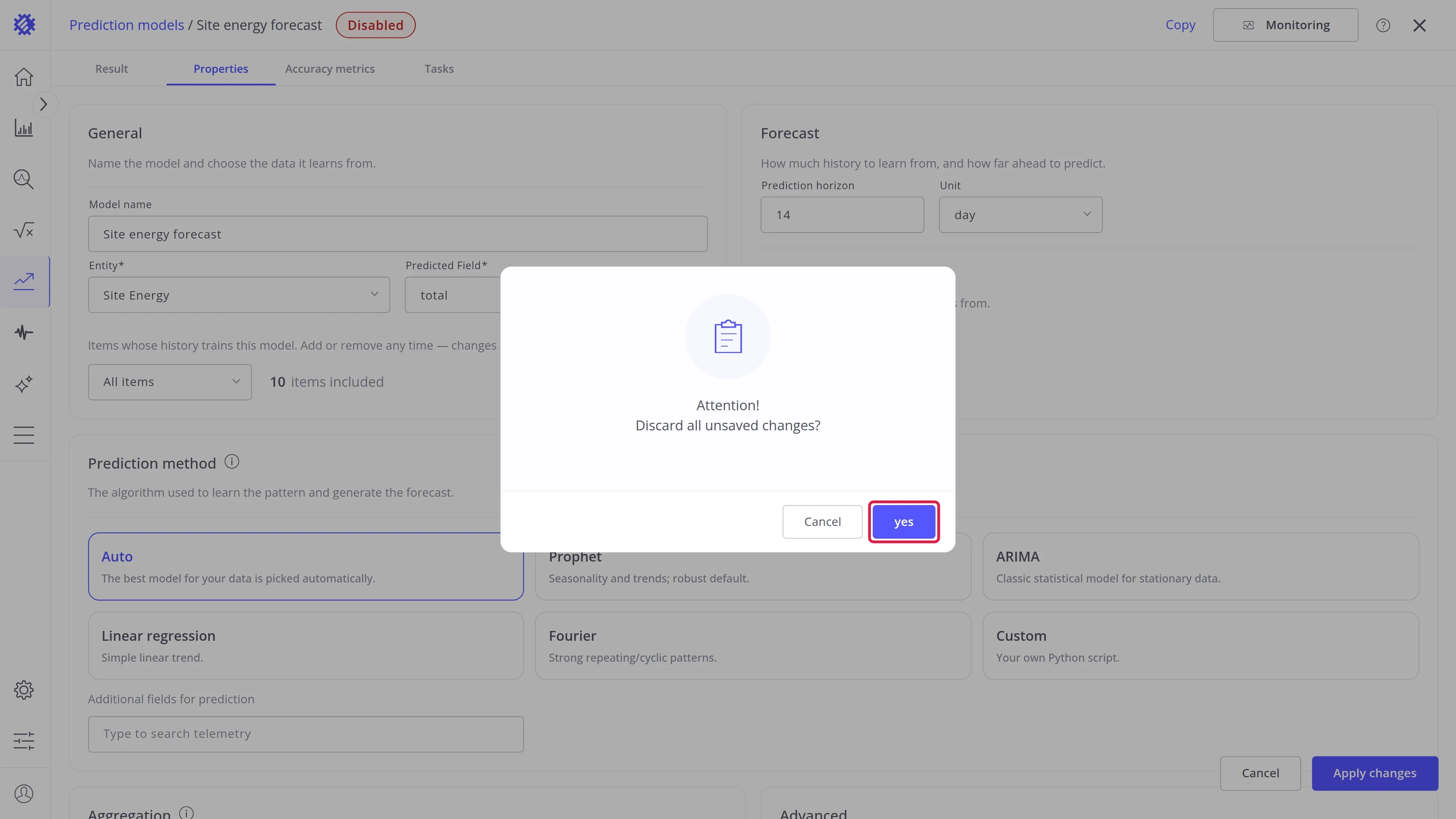
Section titled “Applying changes”Cancel discards your edits. Click yes to go back to the saved settings.
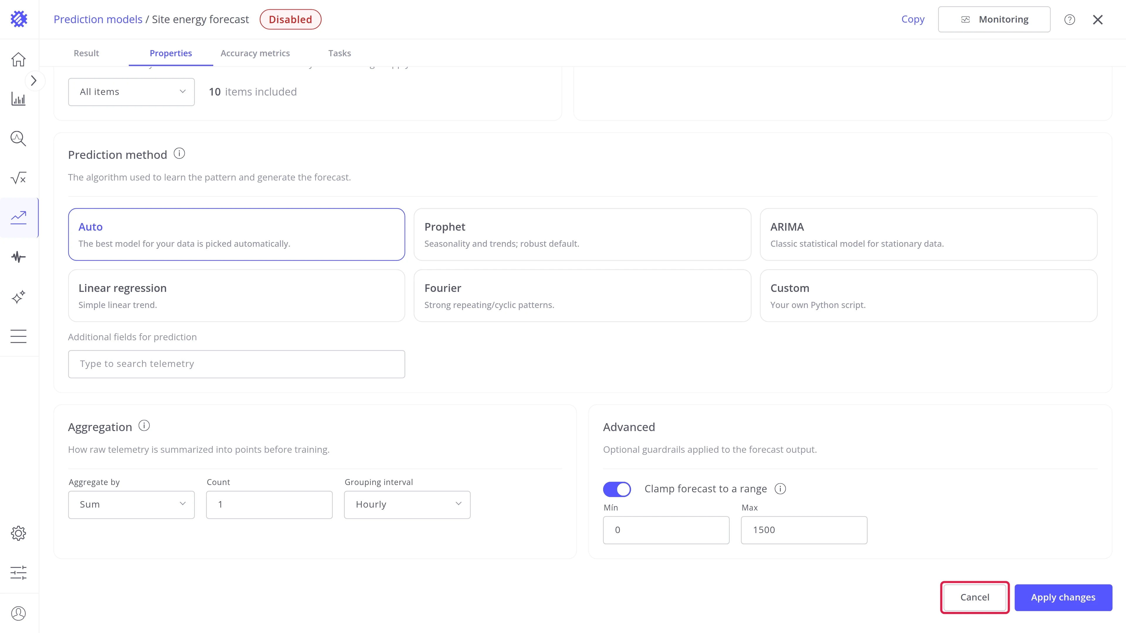
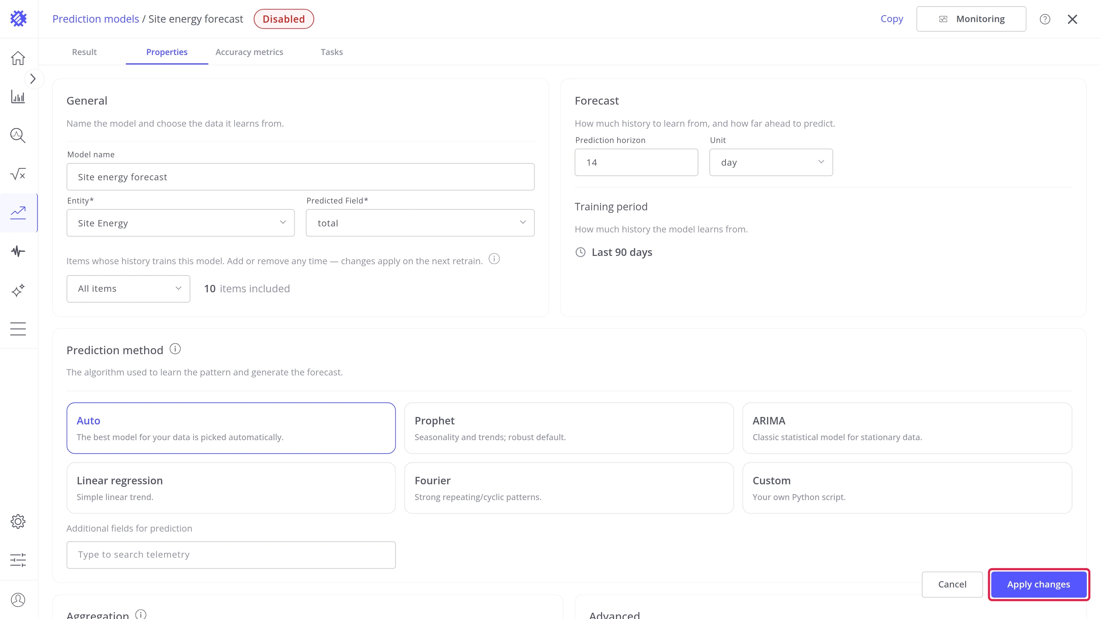
Apply changes saves your edits. If the model has to be trained again, click Rebuild to confirm.
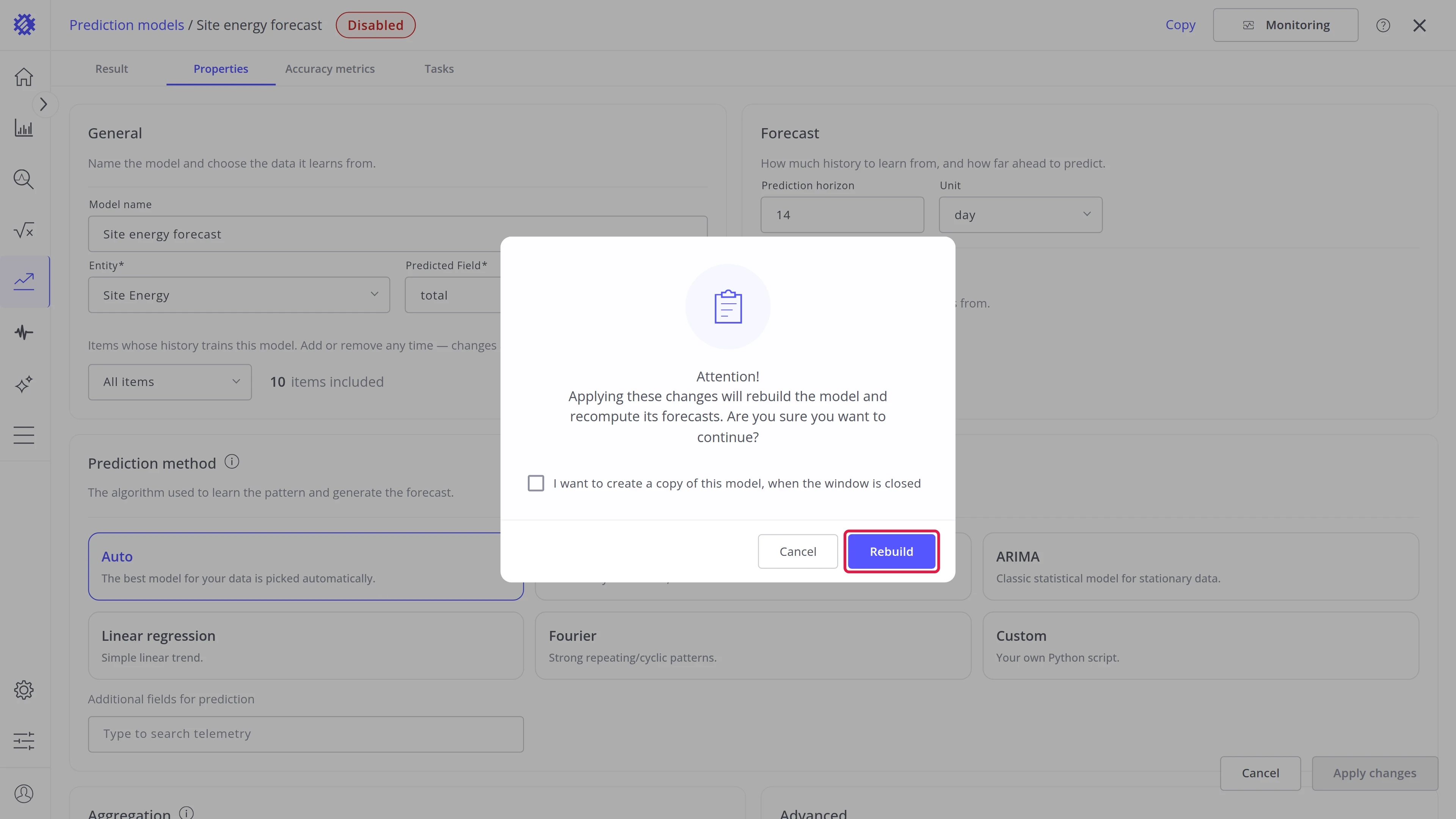
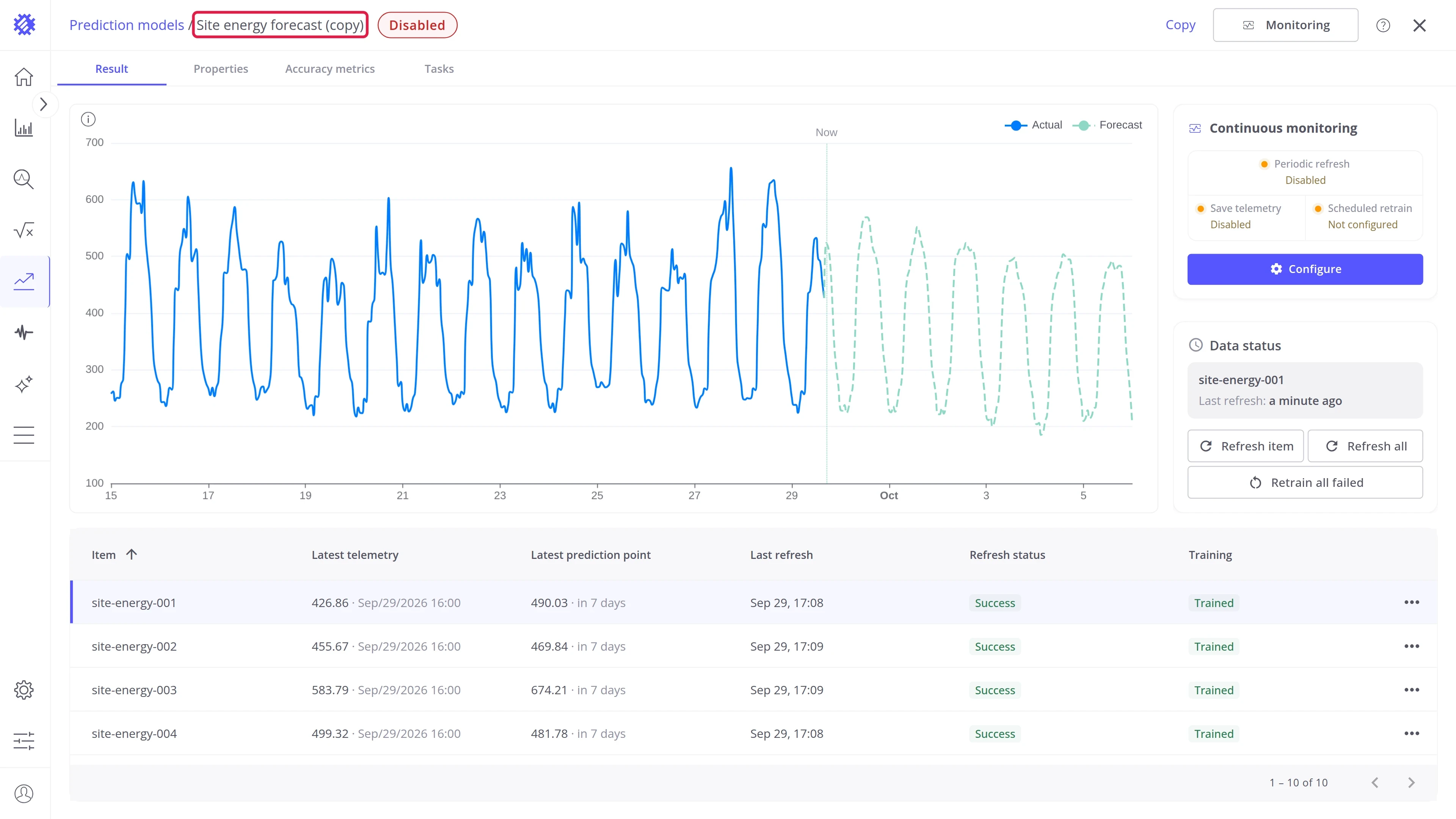
Apply the change to a copy. Use it to try a change without touching this model:
- In the dialog, check I want to create a copy of this model (1).
- Click Create copy (2).
- A new model opens in a new browser tab, named with (copy) at the end. It holds your change and trains on its own.
The original model keeps its settings and forecasts.
Wizard advanced settings
Section titled “Wizard advanced settings”Before you build a model, the wizard lets you also choose its prediction method and limit its forecast. This is optional and works the same for every intent.
Click Advanced settings on the step before the build. The wizard adds one more step with two cards.
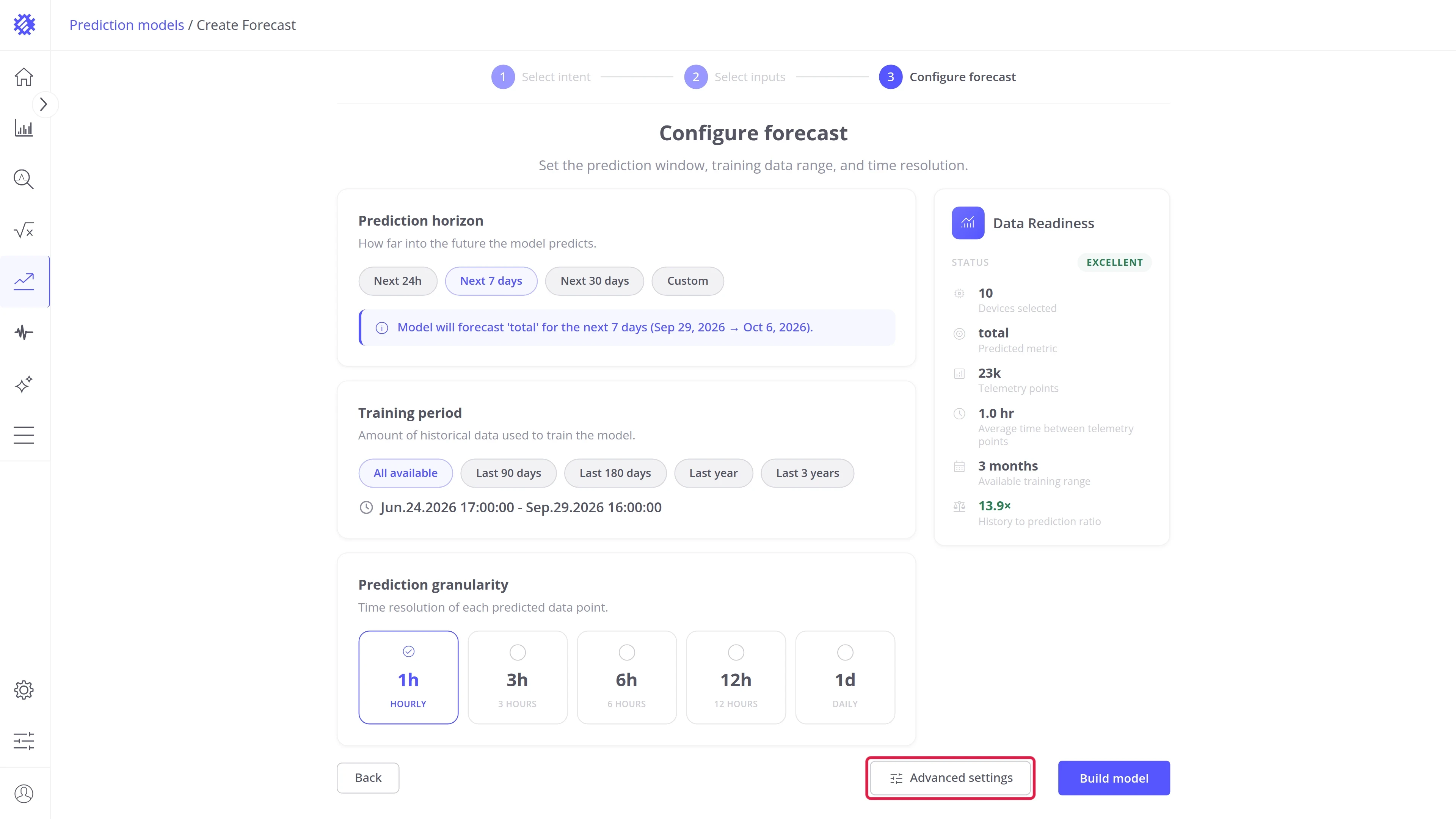
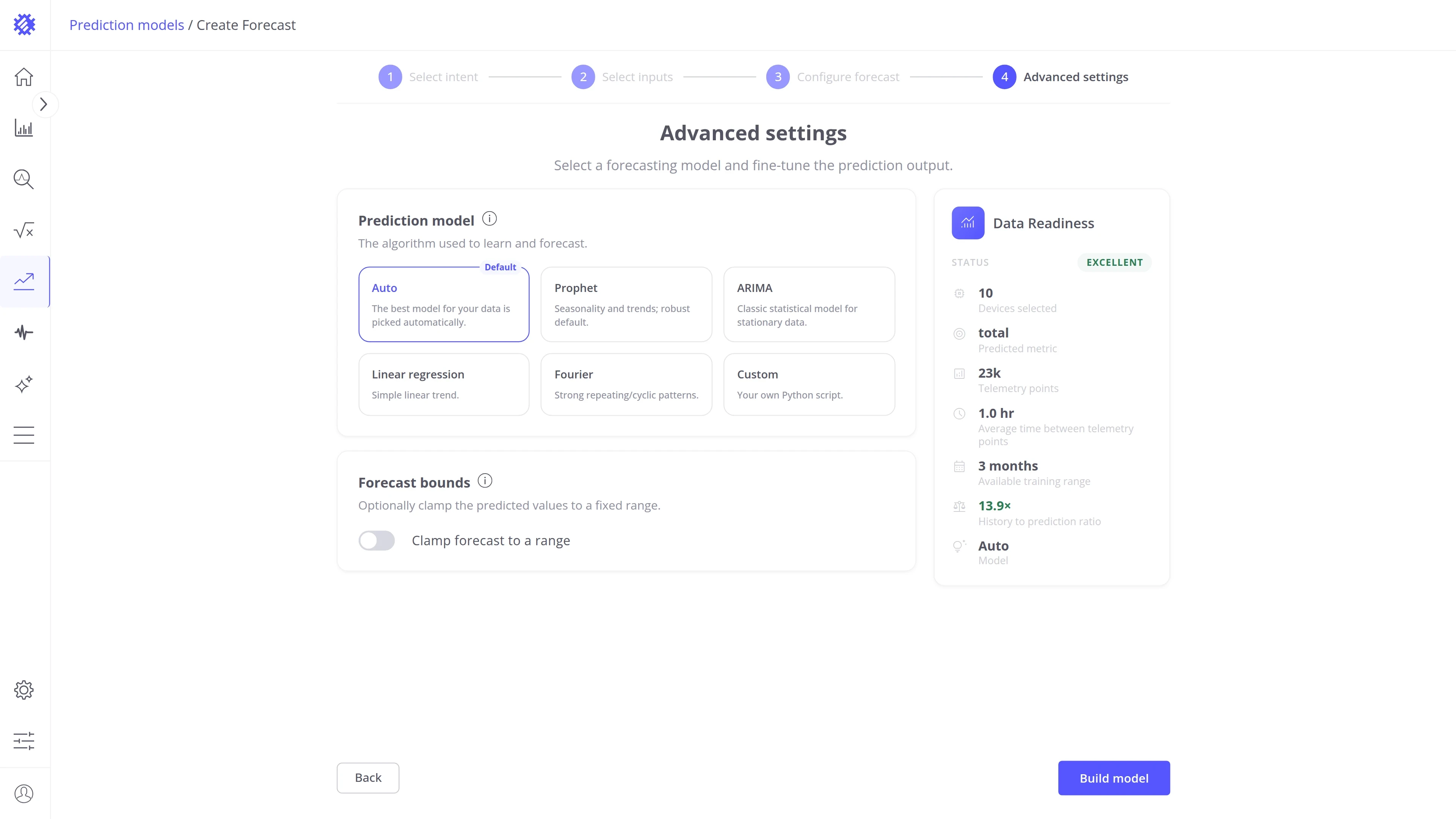
On the first card, Prediction model, choose the algorithm the model learns with. Auto is already selected. The options are the same as on the Prediction method card of the Properties tab.
On the second card, Forecast bounds, switch Clamp forecast to a range on if the forecast must stay between Min and Max, as on the Advanced card of the Properties tab.
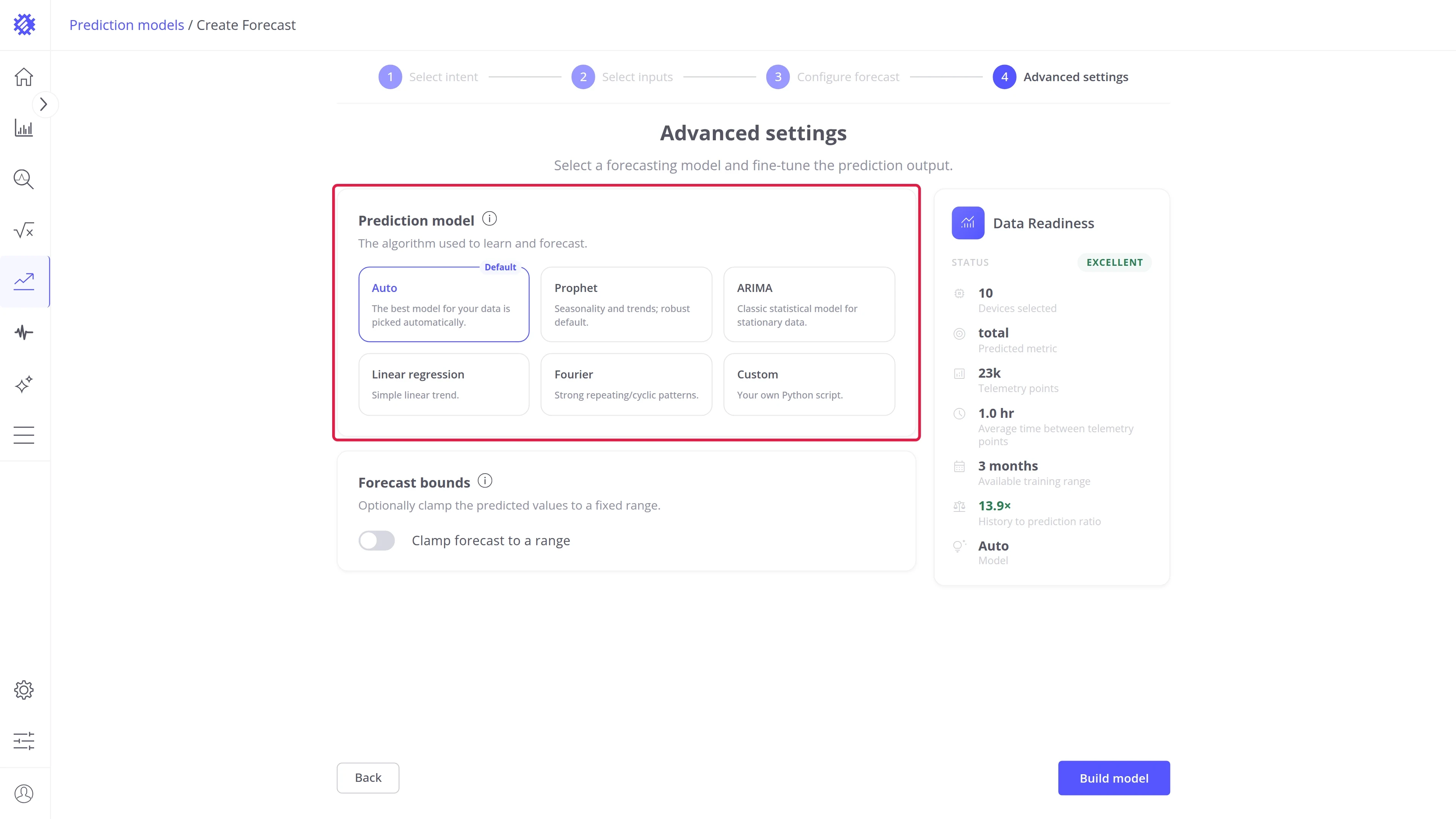
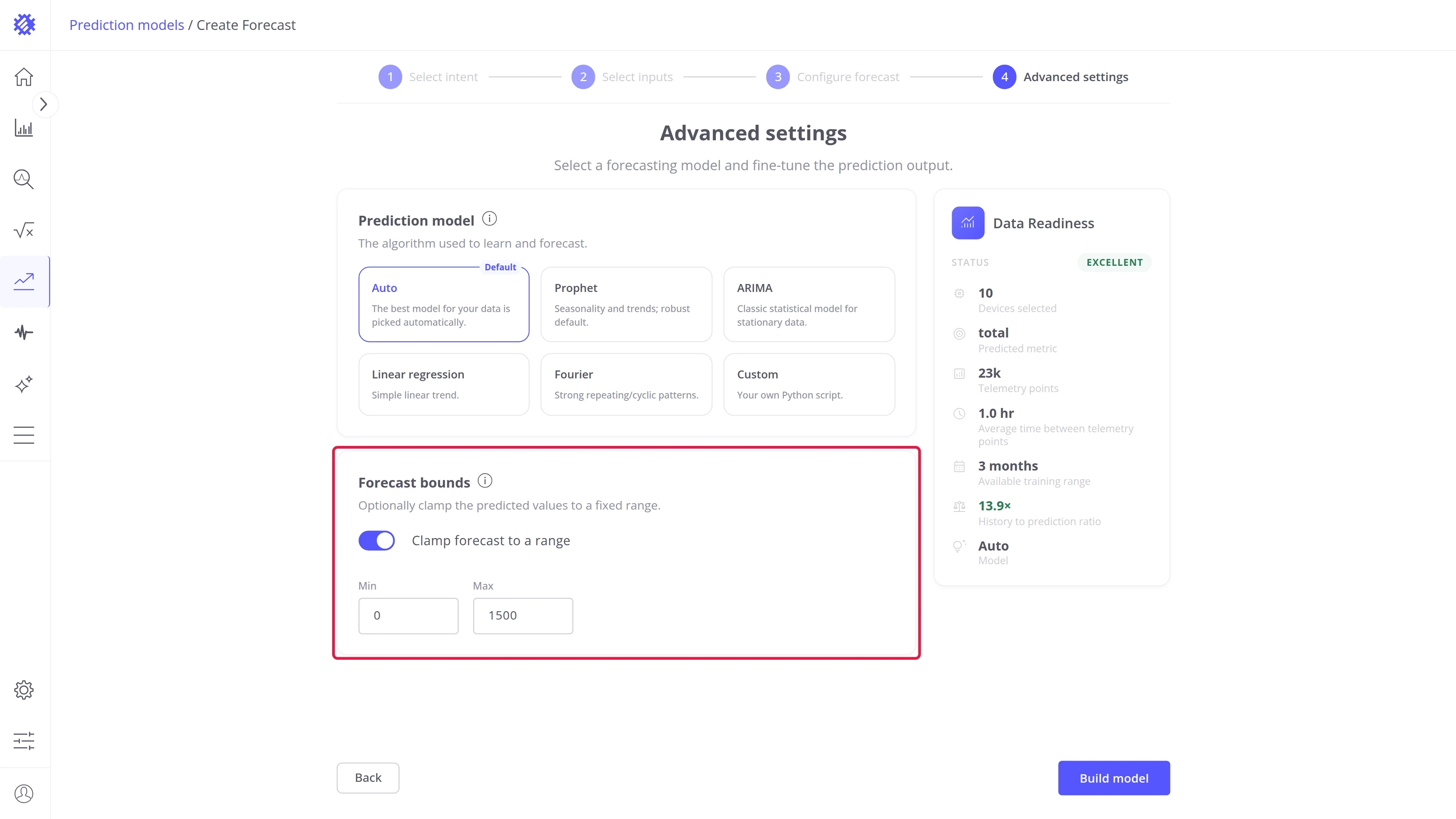
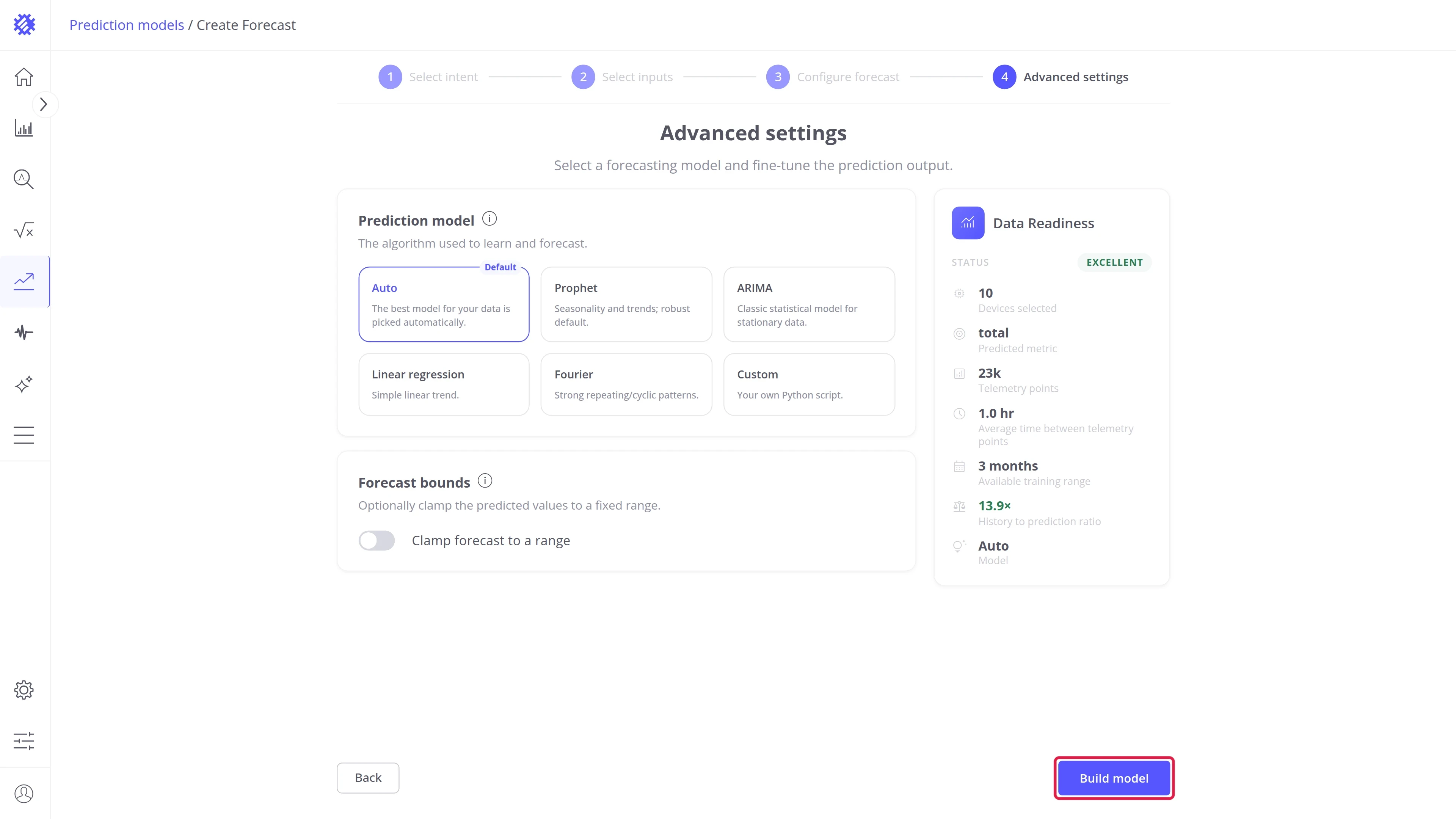
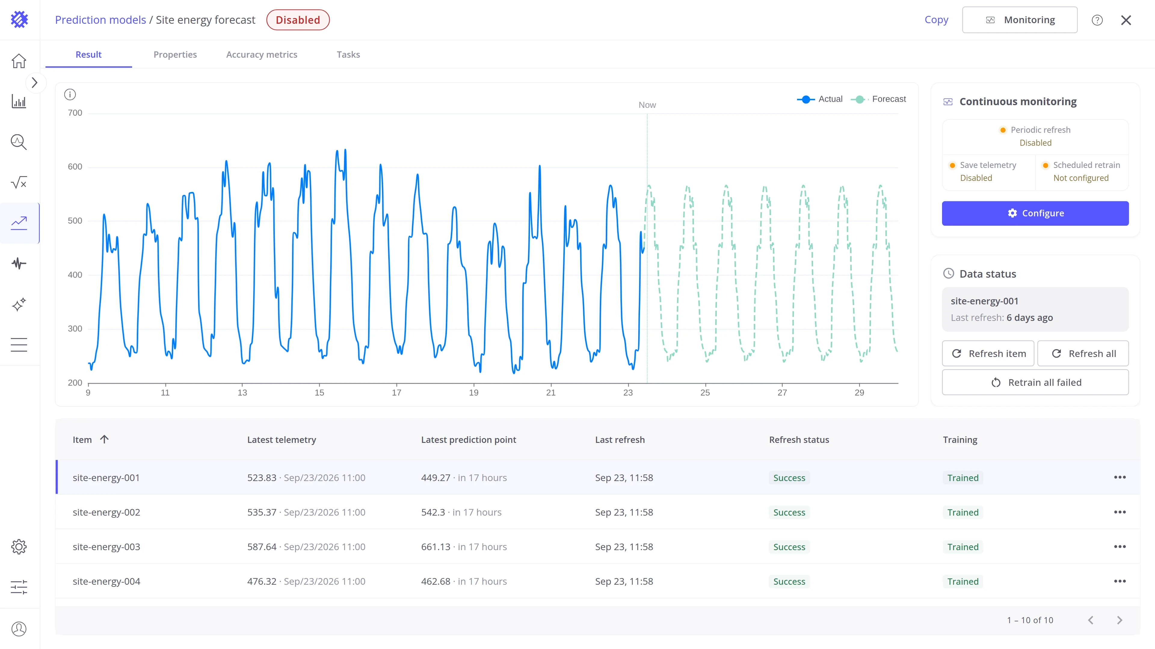
When both cards are set, click Build model. Trendz trains the model and opens its Result tab when training is done.
Prediction methods
Section titled “Prediction methods”The prediction method is the algorithm that learns from the history and makes the forecast. Pick it on the Prediction method card of the Properties tab, or in the wizard advanced settings.
Built-in models
Section titled “Built-in models”| Model | Best for |
|---|---|
| Auto | Most data. Trains Linear regression, Fourier, ARIMA, and Prophet on each device and keeps the most accurate one |
| Prophet | Data with daily, weekly, or yearly patterns and a trend. Handles gaps well |
| ARIMA | A series that follows its own recent past, with trends. p, d, and q set the autoregressive, differencing, and moving-average orders; 1, 1, 1 is a safe start |
| Linear regression | A steady rise or fall, like a filter clogging or a battery draining |
| Fourier | Clean repeating cycles, like a machine that runs the same shifts every day |
Prophet, ARIMA, and custom models run in the Python Executor, a separate service. Linear regression and Fourier run inside Trendz.
Custom models
Section titled “Custom models”Use a custom model when the built-in models do not fit your data. You write the model in Python, with any library, and Trendz feeds it the data, stores what it learned, and publishes its forecast, just like a built-in model.
Select Custom as the method and click Edit script. Restore Template fills the editor with an empty model.
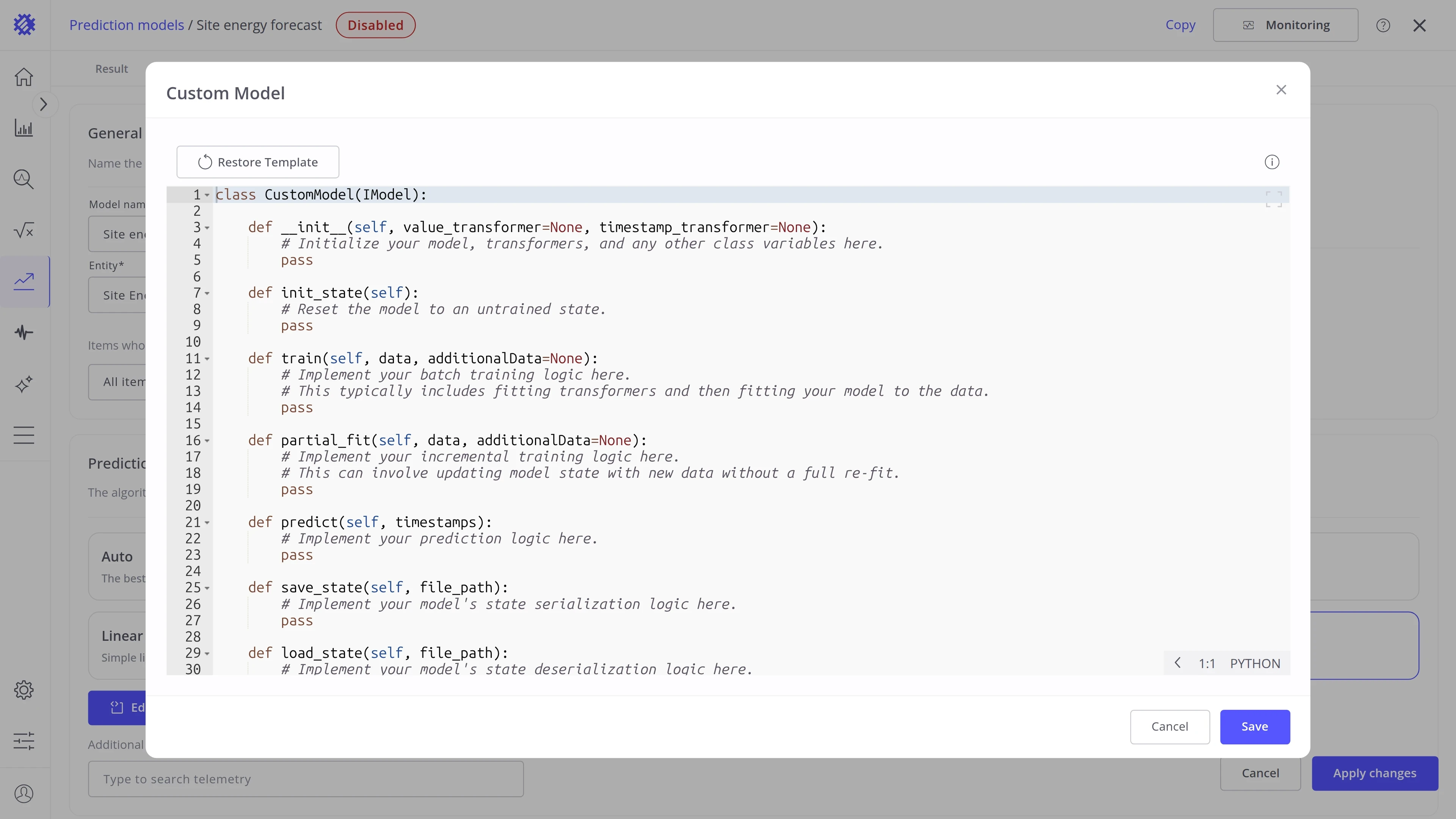
The script defines a class named CustomModel that extends IModel. Trendz provides IModel: do not import it,
and do not rename the class. Trendz calls the methods in this order:
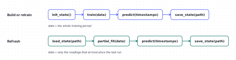
| Method | Called | Purpose |
|---|---|---|
init_state() |
Before a build or retrain | Reset the model |
train(data, additionalData) |
On a build or retrain | Learn from the whole training period |
partial_fit(data, additionalData) |
On a refresh | Learn from the new readings only |
predict(timestamps, additionalData) |
After every train or partial fit | Return one value per timestamp |
save_state(file_path) |
At the end of every run | Write what the model learned to the file |
load_state(file_path) |
At the start of a refresh | Read it back |
name() |
For logs | Return a name for the model |
Everything the model knows must be saved in save_state and read in load_state. Nothing else is kept between
runs.
Input and output. data is a list of [timestamp, value] pairs, oldest first, one per grouping interval.
Timestamps are in milliseconds.
data = [[1719792000000, 412.5], [1719795600000, 398.1], [1719799200000, 405.7]]additionalData holds the additional fields, keyed telemetry_<field id>, in the same format. It is empty when
the model has none.
additionalData = {'telemetry_4f1c2a90_...': [[1719792000000, 21.4], [1719795600000, 20.9]]}predict receives the timestamps to forecast and returns one value for each:
def predict(self, timestamps, additionalData=None): return [self.level for ts in timestamps]Example. A complete model: the average value for each hour of the day, over the last 30 days.
import json
import numpy as np
class CustomModel(IModel):    """Average value per hour of day, over a rolling 30-day buffer."""
    BUFFER_POINTS = 24 * 30
    def __init__(self):        self._buffer = []        self._profile = {}
    def init_state(self):        self._buffer = []        self._profile = {}
    def train(self, data, additionalData=None):        self._buffer = [list(point) for point in data][-self.BUFFER_POINTS:]        self._fit()
    def partial_fit(self, data, additionalData=None):        known = {int(point[0]) for point in self._buffer}        fresh = [list(point) for point in data if int(point[0]) not in known]        self._buffer = sorted(self._buffer + fresh, key=lambda point: point[0])[-self.BUFFER_POINTS:]        self._fit()
    def predict(self, timestamps, additionalData=None):        fallback = float(np.mean([point[1] for point in self._buffer])) if self._buffer else 0.0        return [self._profile.get(self._hour(ts), fallback) for ts in timestamps]
    def save_state(self, file_path):        state = {'buffer': self._buffer, 'profile': {str(h): v for h, v in self._profile.items()}}        with open(file_path, 'w') as f:            json.dump(state, f)
    def load_state(self, file_path):        with open(file_path) as f:            state = json.load(f)        self._buffer = state['buffer']        self._profile = {int(h): v for h, v in state['profile'].items()}
    def name(self):        return 'hour-of-day-mean'
    def _fit(self):        by_hour = {}        for ts, value in self._buffer:            by_hour.setdefault(self._hour(ts), []).append(value)        self._profile = {hour: float(np.mean(values)) for hour, values in by_hour.items()}
@staticmethod def _hour(ts): return int(ts // 3600000) % 24Packages. The Python Executor includes numpy, pandas, scikit-learn, statsmodels, matplotlib,
prophet, xgboost, and requests. To add others to a self-hosted executor, see
Add custom Python libraries.
Accuracy
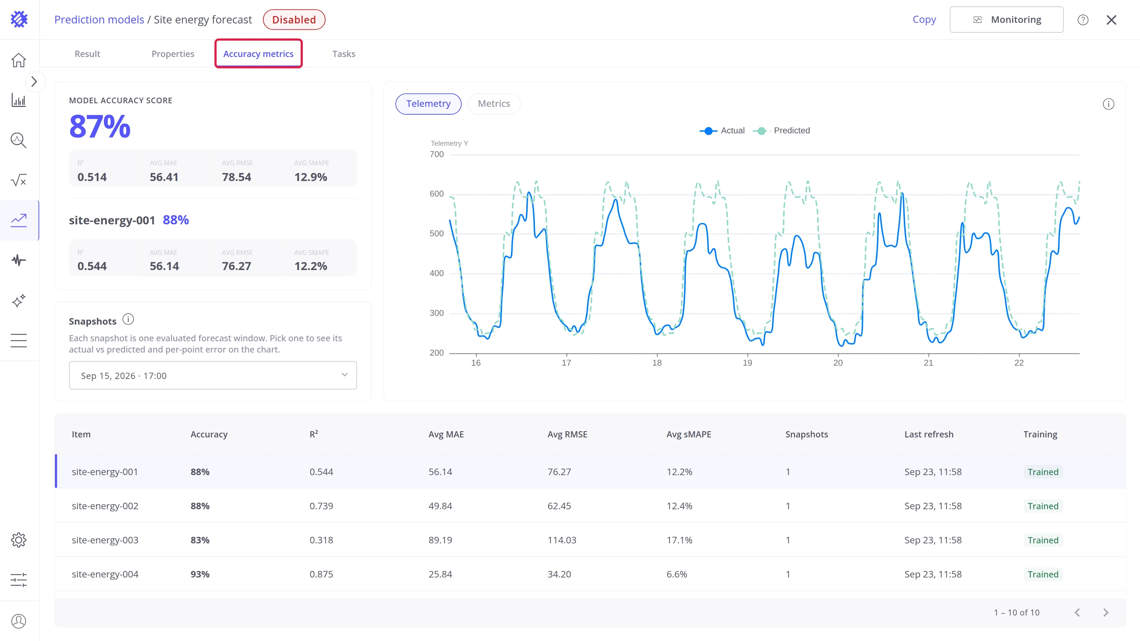
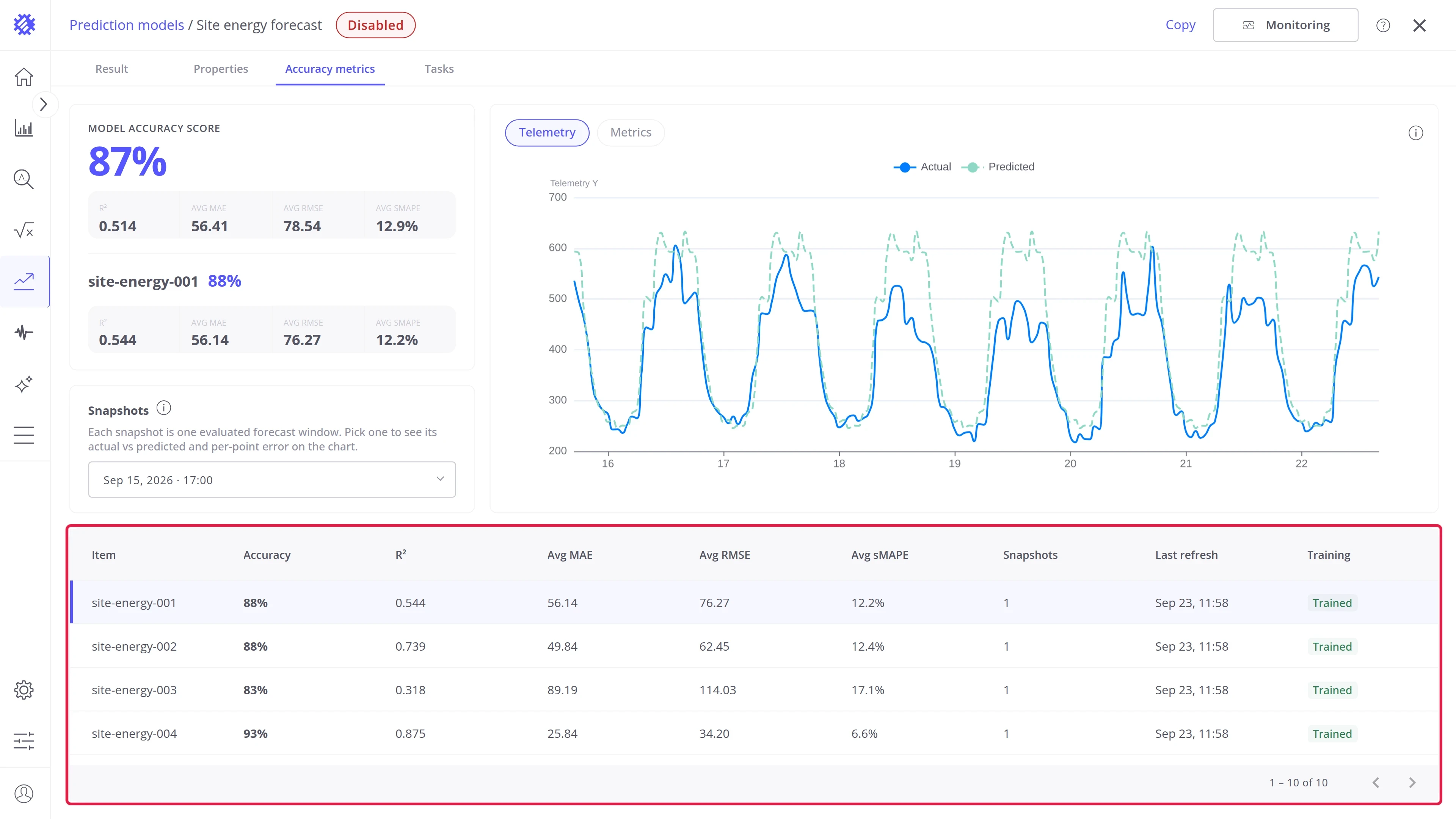
Section titled “Accuracy”The Accuracy metrics tab shows how close the forecasts came to what really happened, for the whole model and for each item.
How accuracy is measured
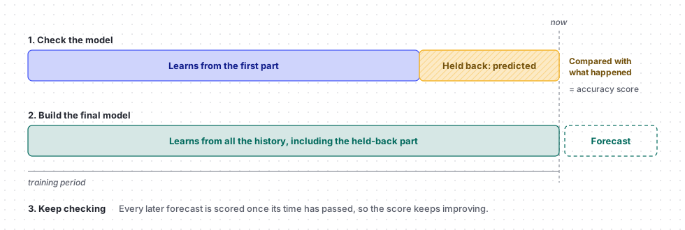
Section titled “How accuracy is measured”To know how accurate a model is, its predicted values have to be compared with the real ones. Trendz does this by answering two questions. For example, for a model that predicts 7 days ahead:
- How accurate would the forecast have been 7 days ago? Right after training, Trendz hides the last 7 days of history, predicts them as if they had not happened yet, and compares the forecast with the real readings. This gives the first score. Then Trendz trains the final model on all the history, including the hidden 7 days, so no data is lost.
- How accurate is the forecast made now? That is known only once the next 7 days of readings arrive. Trendz stores the forecast as a snapshot and compares it with the real readings when they come in. Every refresh does the same, so the score keeps up with the newest data.
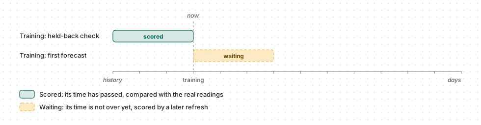
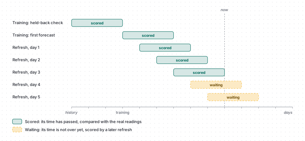
A snapshot is one forecast of one item, one horizon long, stored at the moment it was made. Snapshots are how the score keeps up with the newest data:
- Training stores two snapshots: the held-back check, scored at once, and the first forecast.
- Every refresh stores its new forecast as another snapshot.
- Once its time has passed, the next refresh compares the snapshot with the real readings.
Accuracy = 100 − sMAPE, from 0 to 100 %. sMAPE is the average error in percent, so 90 % means the forecast was off by about 10 % on average.
An item needs at least twice the prediction horizon of history: one part to learn from and one to check. An item with less still forecasts, and gets a score once enough history arrives.
Layout
Section titled “Layout”To open the tab, click Accuracy metrics in the tabs of the model page.
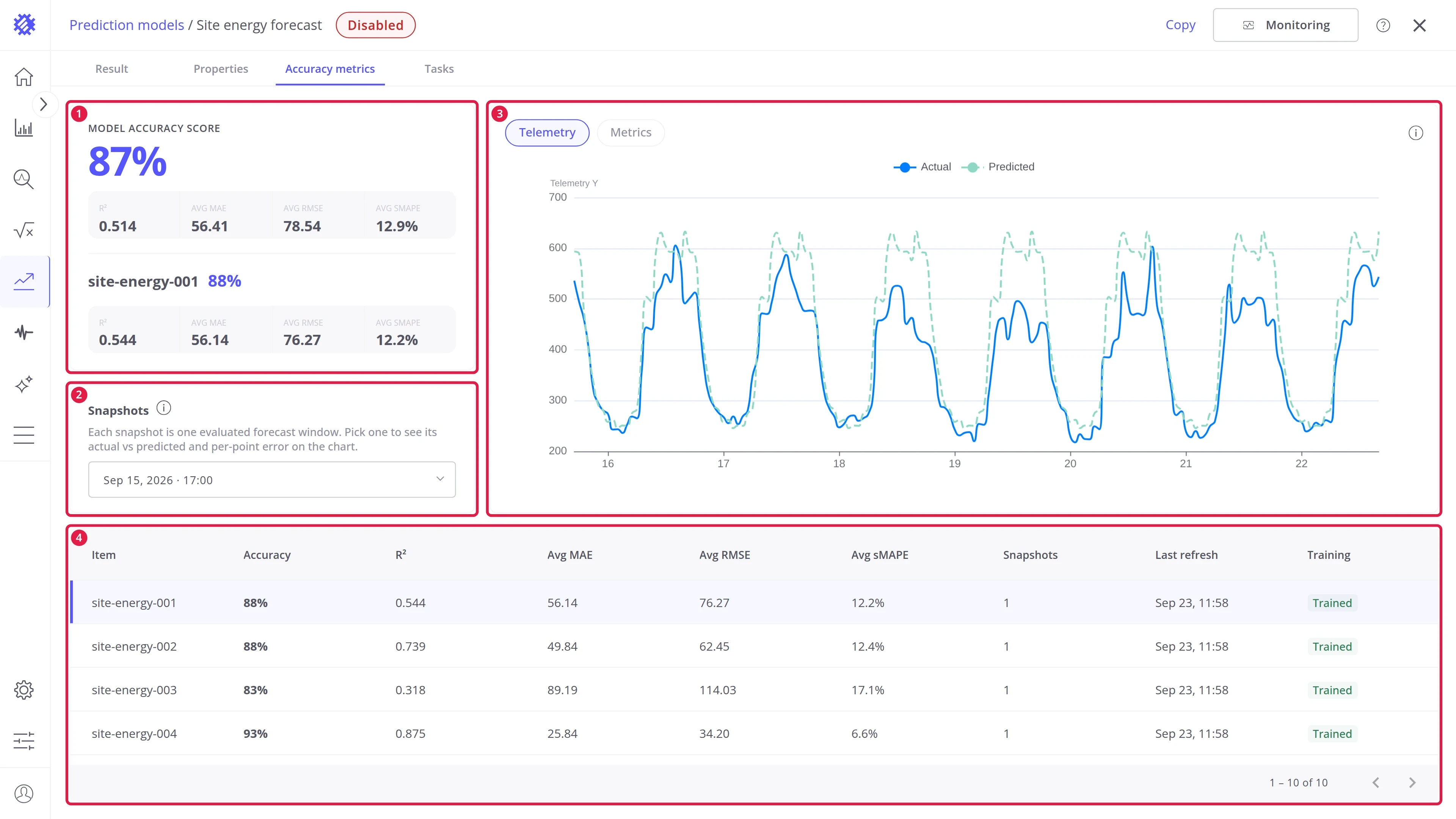
| # | Area | Contents |
|---|---|---|
| 1 | Score | The accuracy of the model, and of the selected item |
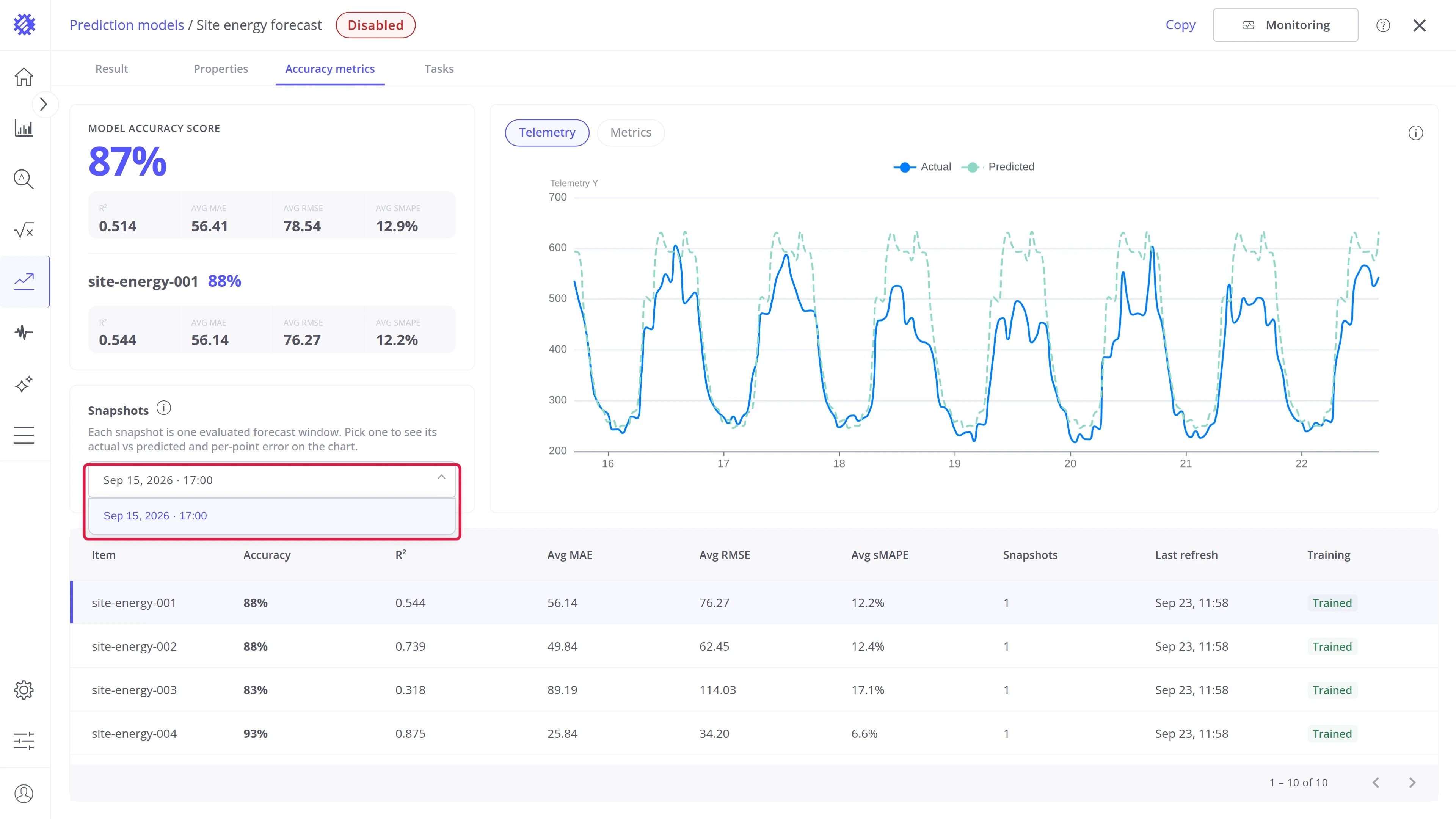
| 2 | Snapshots | The checked forecasts, to pick one for the chart |
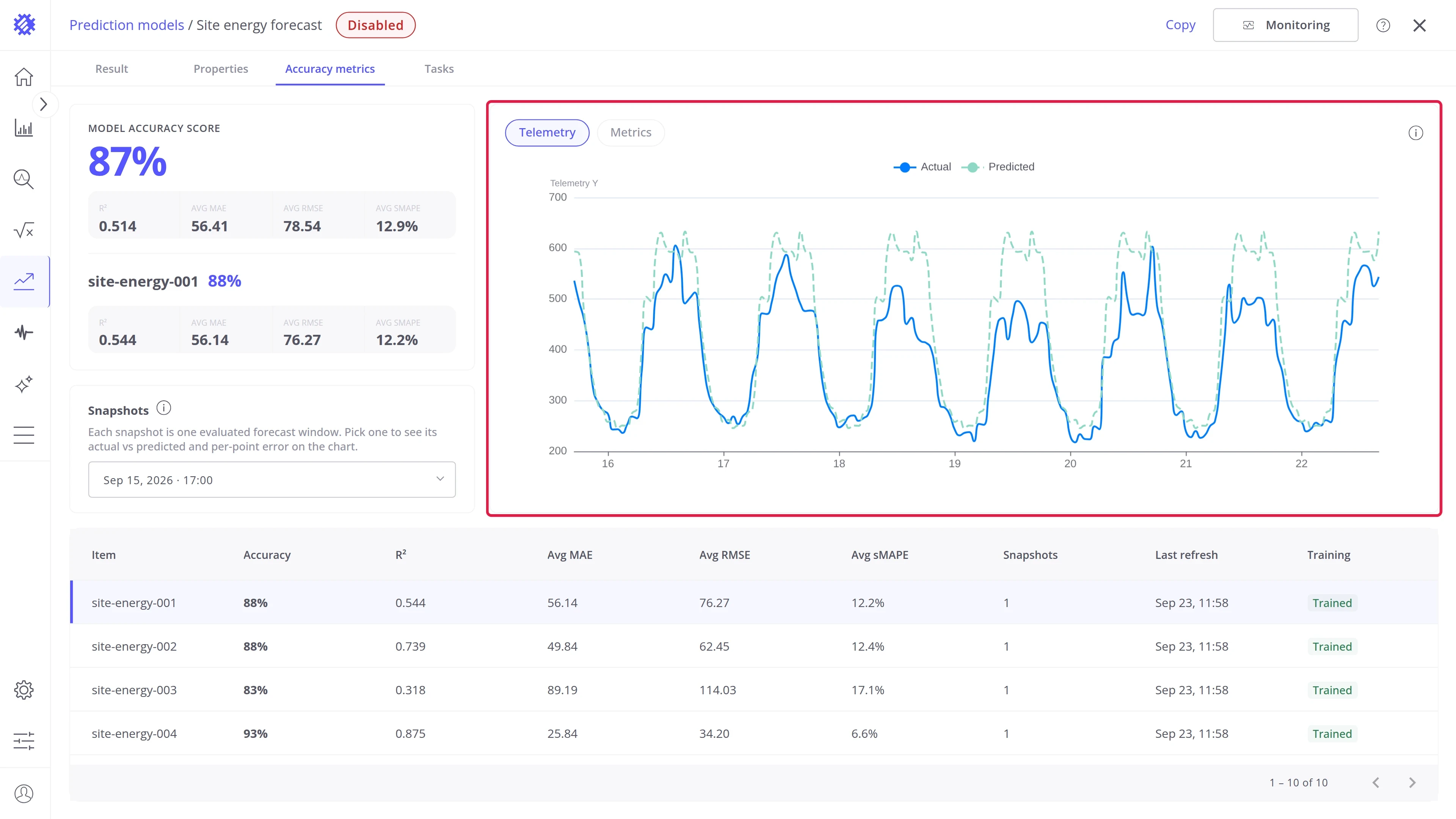
| 3 | Chart | The picked snapshot: actual against predicted, or the error at each point |
| 4 | Items table | Every item with its own score |
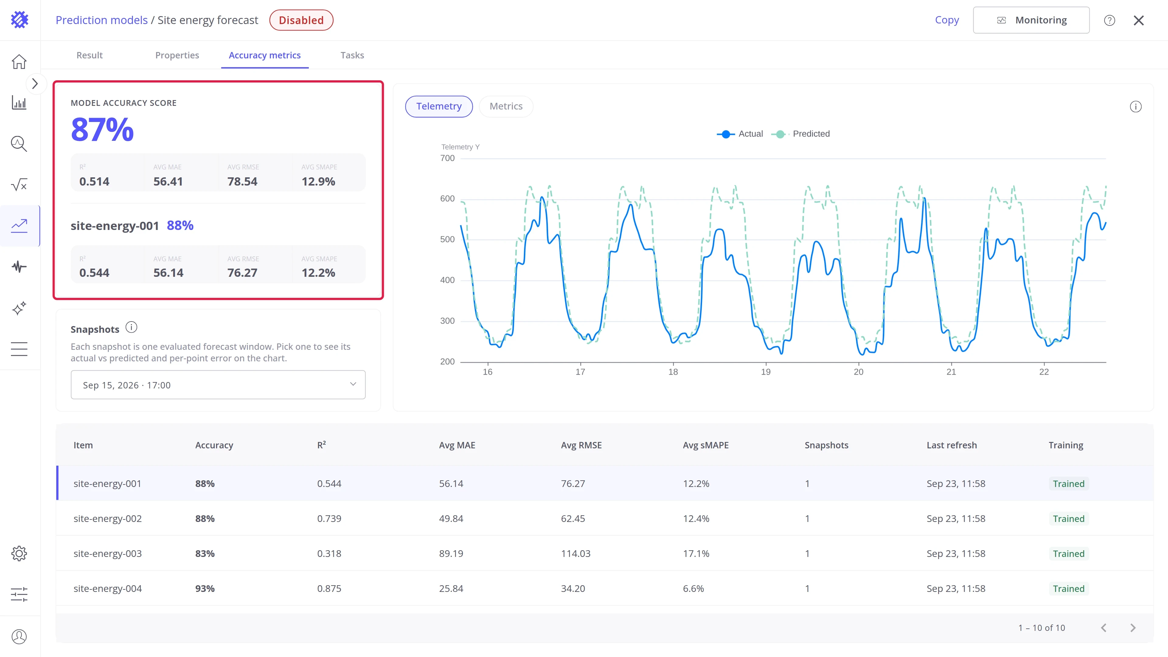
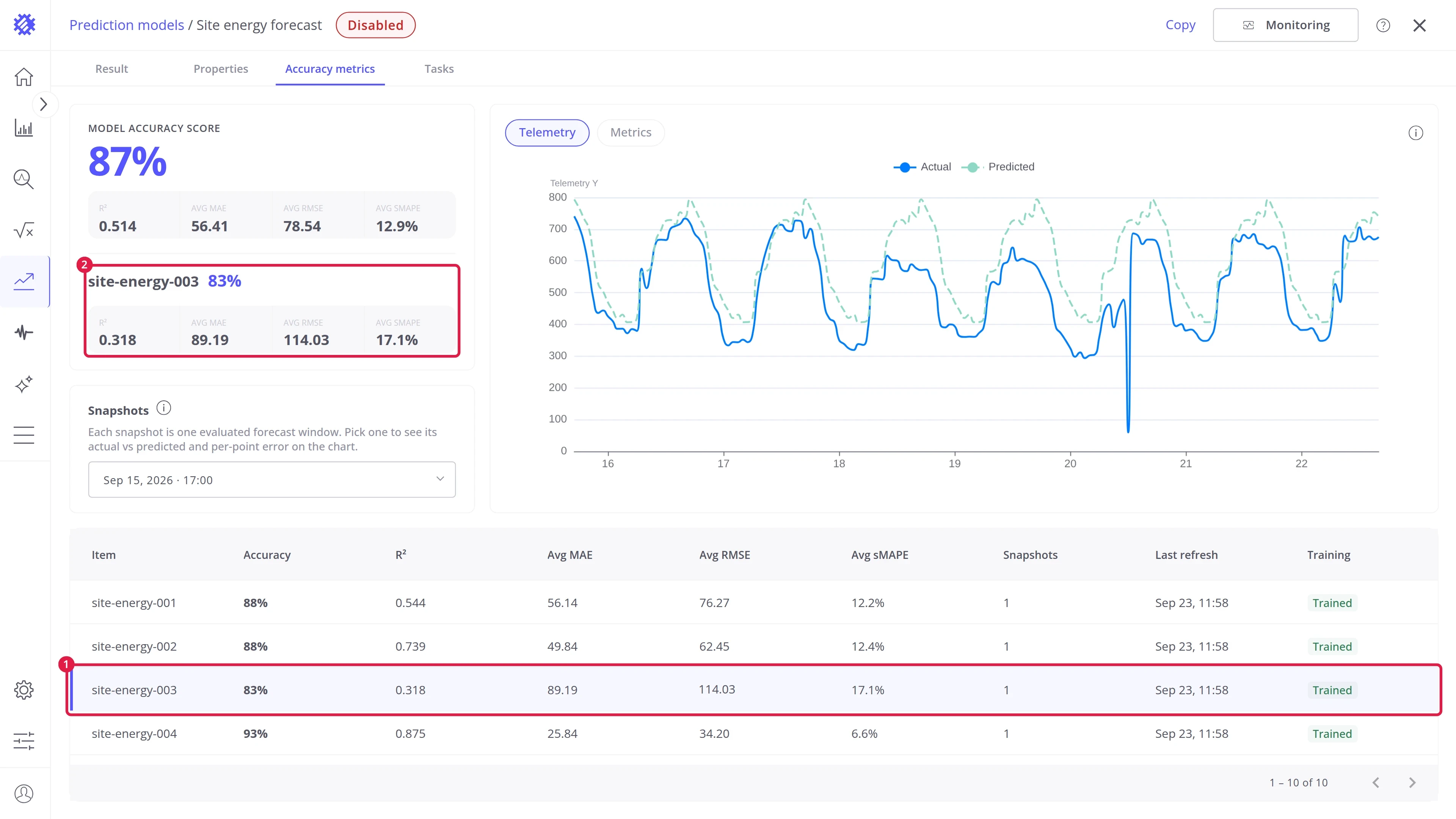
The top shows the Model accuracy score, for all items together. Below it is the score of the item selected in the table. Each has four more numbers:
| Metric | What it says |
|---|---|
| R² | How much of the change in the data the model explains. Closer to 1 is better |
| Avg MAE | The average error, in the units of the data |
| Avg RMSE | Like MAE, but big misses count more |
| Avg sMAPE | The average error in percent |
Snapshots
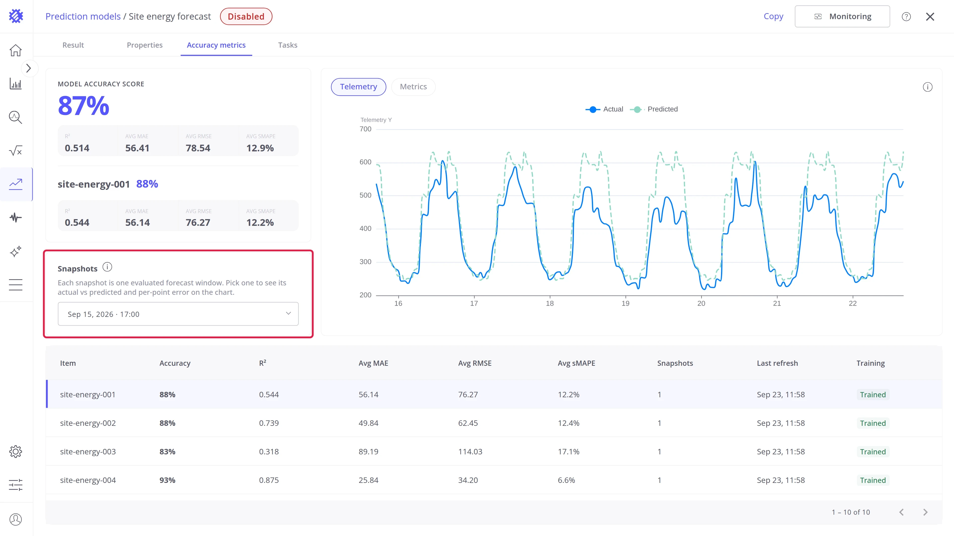
Section titled “Snapshots”The card lists the scored snapshots, and the score of the item is built from them. Trendz keeps the last 100 snapshots of each item. Without Periodic refresh, set in Monitoring & Alarms, no new forecasts are scored, and the list holds only the check from training.
Pick a snapshot to draw it on the chart.
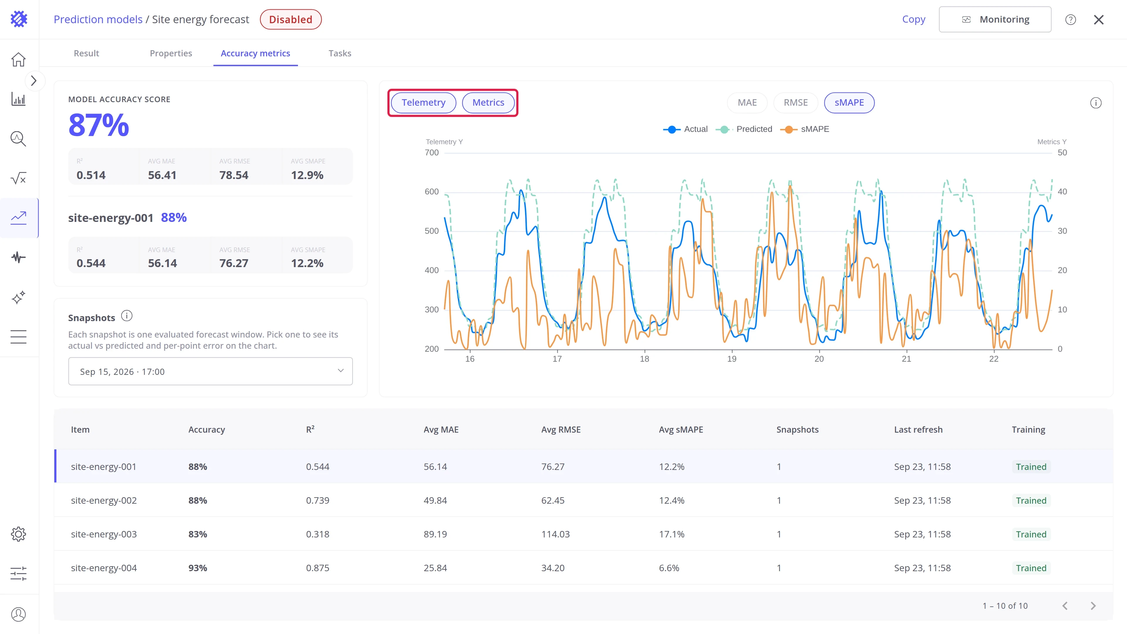
The chart shows the picked snapshot of the selected item. Two switches above it choose what to draw, one or both at once:
- Telemetry: the actual and the predicted values. On by default.
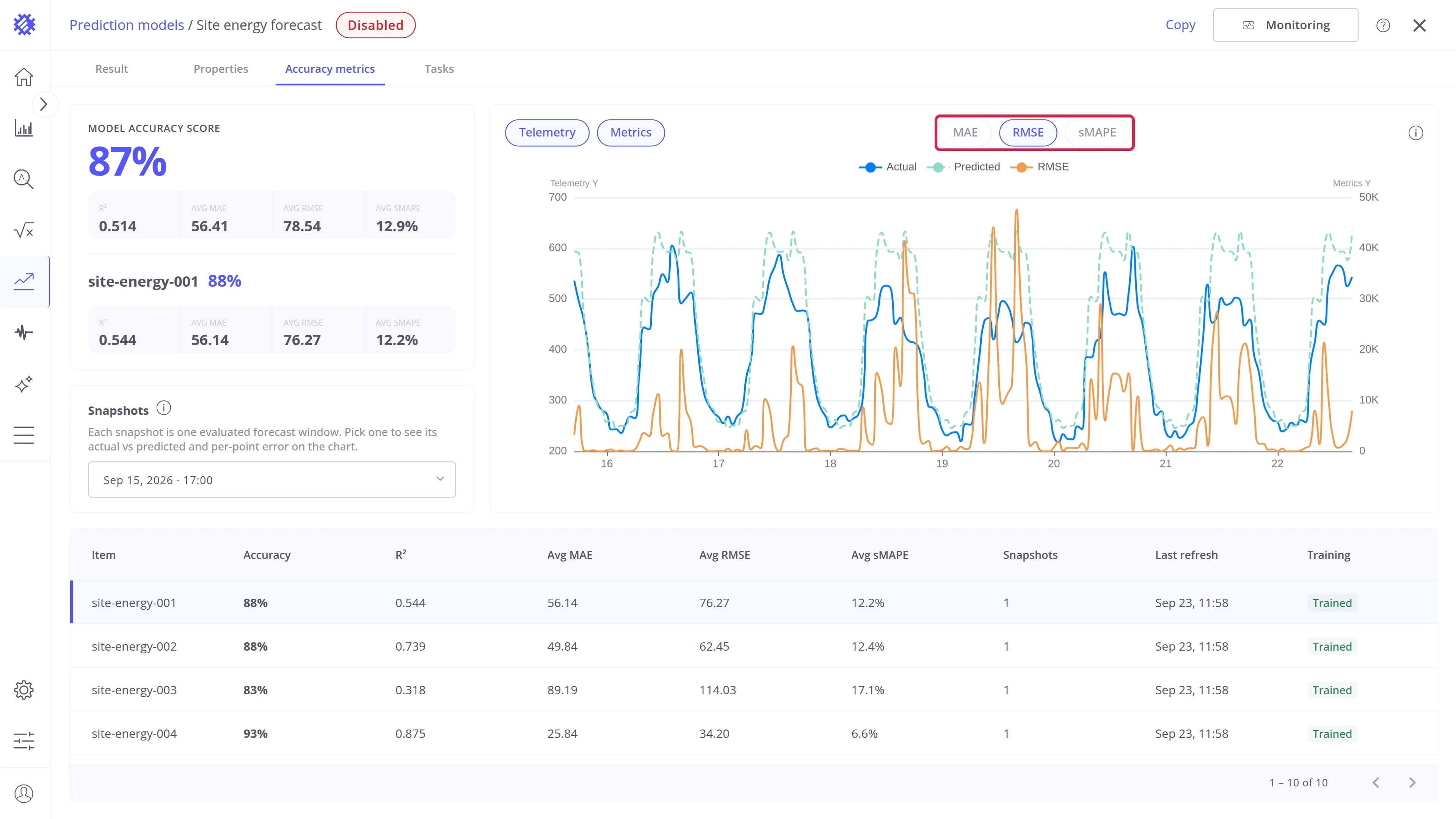
- Metrics: the error at each point. When it is on, pick which error to draw: MAE, RMSE, or sMAPE.
Items table
Section titled “Items table”Every item of the model with its Accuracy, R², Avg MAE, Avg RMSE, Avg sMAPE, the number of Snapshots, the Last refresh, and its Training status. Click a row (1) to show that item in the score card (2) and on the chart.
Improve accuracy
Section titled “Improve accuracy”- Give the model more history.
- Use a longer grouping interval, for example hours instead of minutes.
- Shorten the prediction horizon.
- Add a field that explains the predicted one.
- Go back to Auto if you picked a method by hand.
- Turn on Scheduled retrain, so the model keeps up with the device.
Where to go next
Section titled “Where to go next”Explore intents
Section titled “Explore intents”-
Forecast
Predict the next values of a metric, like the energy of the next 7 days.
-
Time to Threshold
Predict when a metric crosses a limit, and raise an alarm before it happens.
-
Period Total
Predict the total, peak, or average of a period, such as the energy of this month.
-
Hit Target
Predict whether a goal is reached by the end of a period, and how far off it is.
Explore more
Section titled “Explore more”Was this helpful?